Week 7 - Simulation of a 1D Super-sonic nozzle flow simulation using Macormack Method
1D Quasi subsonic-supersonic isentropic nozzle flow:
let us consider a convergent-divergent nozzle as below
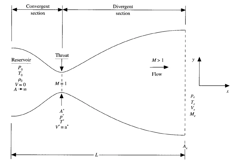
Consider a one dimensional steady isentropic flow through this nozzle.
The flow at inlet of the nozzle comes from a reservoir where the flow field variables are
`rho_o = density; T_o = temperature, p_o = pressure`. Area be `A_o`
let the exit pressure, temperature, velocity and mach number be `p_e, T_e, V_e and M_e` respectively`
let the velocity, temperature, pressure and density at the throat area be `V^*, T^*, p^*and `rho_*``respectively`. Area be `A^*`
Velocity, temperature, pressure and density are called primitive variables (flow field variables).
lets assume that at a given section, the flow properties are constant. This means that although the flow is two dimensional, the flow properties vary only in X direction. The flow is uniform in Y direction. Thsi type of flow is called Quasi one dimensional flow.
The governing equations for quasi 1D steady isentropic flow are expressed as
Continuity: `rho_1*V_1*A_1 = rho_2*V_2*A_2`---> (1)
Momentum : `p_1*A_1 + rho_1*V_1^2*A_1 + int_(A_1)^(A_2)pdA = p_2A_2 + rho_2*V_2^2*A_2` ---> (2)
Energy : `h_1 + V_1^2/2 = h_2 + V_2^2/2` ---> (3)
where subscripts 1 and 2 denote different locations along the nozzle.
Also, `p = rho*R*T` ---> (4) which is perfect gas equation and
`h = C_p*T` ---> (5) is the enthalpy
The above equations can be solved analytically for the flow through the nozzle.
Nozzle area distribution:
The nozzle shape is chosen to be a parabolic area distribution given by
`A = 1 + 2.2(x-1.5)^2` where `0<=x<=3` ---> (6)
Non dimensionalisation:
For simplification in comparing the values at different locations, let us non dimensionalize the fluid flow variables, time and area with respect to reservoir values.
Therefore,
non dimensional density is `rho^' = rho/rho_o`
non dimensional temperature is `T^' = T/T_o`
non dimensional pressure is `p^' = p/p_o`
non dimensional velocity is `V^' = V/a_o where a_o = velocity of sound= sqrt(gamma*R*T_o)`
non dimensional length is `x^' = x/L`
non dimensional area `A^' = A/A^*` where `A^* =`area at throat
non dimensional time `t^' = t/(L/a_o)`
Non conservation form of governing equations:
Continuity:
`(del(rho*A))/(delx) + rho*A*(delV)/(delx) + rho*V*(delA)/(delx) + V*A*(delrho)/(delx) = 0` --->(7)
Momentum:
`rho*(delV)/(delt) + rho*V*(delV)/(delx) = -R*(rho*(delT)/(delx) + T*(delrho)/(delx))` ---> (8)
Energy:
`rho*C_v*(delT)/(delx) + rho*V*C_v*(delT)/(delx) = -rho*R*T*((delV)/(delx) + V*(del(lnA))/(delx))` ---> (9)
Converting the above equations to non dimensionalized form
Continuity:
`(delrho^')/(delt^') = -rho^'*(delV^')/(delx^') - rho^'*V^'*(del(lnA))/(delx^') - V^'*(delrho^')/(delx^')` ---> (10)
Momentum:
`(delV^')/(delt^') = -V^'*(delV^')/(delx^') - (1/gamma)*((delT^')/(delx^') + (T^'/rho^')*(delrho^')/(delx^'))` ---> (11)
Energy:
`(delT^')/(delt^') = -V^'*(delT^')/(delx^') - (gamma-1)*T^'*((delV^')/(delx^') + V^'*(del(lnA^'))/(delx^'))` ---> (12)
The above equations can be solved numerically using time marching technique.
Initial conditions:
To solve equations using time marching, initial values at time t = 0 for density, velocity and temperature must be setup. For simplicity, it is assumed that the flow field variables vary linearly with x.
Therfore, at time t=0,
`rho = 1-0.3146*x`
`T = 1-0.2314*x`
`V = (0.1+1.09*x)*T^0.5`
Boundary conditions:
Based on the method of characteristics study,
at inflow boundary which is subsonic, two flow field variables must be specified and one flow field variable must be float (varying).
Point 1, being the reservoir, density and temperature (non dimensional) are specified. These are held fixed independent of time. Also, velocity is allowed to float.
Therefore, at point 1,
`V_1 = 2*V_2 - V_3`
`rho_1 = 1`
`T_1 = 1`
At outflow boundary which is supersonic, all flow fiedl variables are allowed to float.
Therefore, at point N,
`V_N = 2*V_(N-1) - V_(N-2)`
`rho_N = 2*rho_(N-1) - rho_(N-2)`
`T_N = 2*T_(N-1) - T_(N-2)`
Conservation form of governing equations:
Continuity:
`(del(rho*A))/(delt) + (del(rho*A*V))/(delx) = 0` ---> (13)
Momentum:
`(del(rho*A*V))/(delt) + (del(rho*A*V^2))/(delx) = -A*(delp)/(delx)` ---> (14)
Energy:
`(del(rho*(e+V^2/2)*A))/(delt) + (del(rho*(e+V^2/2)*A*V+p*A*V))/(delx) = 0` ---> (15)
Converting the above equations to non dimensionalized form
Continuity:
`(del(rho^'*A^'))/(delt^') + (del(rho^'*A^'*V^'))/(delx^') = 0` ` ---> (16)
Momentum:
`(del(rho^'*A^'*V^'))/(delt^') + (del(rho^'*A^'*(V^')^2+(1/gamma)*p^'*A^'))/(delx^') = (1/gamma)*p^'*(delA^')/(delx^')` ---> (17)
Energy:
`(del(rho^'*(e^'/(gamma-1)+gamma*(V^')^2/2)*A^'))/(delt^') + (del(rho^'*(e^'/(gamma-1)+gamma*(V^')^2/2)*A^'*V^'+p^'*A^'*V^'))/(delx^') = 0` ---> (18)
In general, the generic form of governing equations for 1D can be written as
`(delU)/(delt) + (delF)/(delx) = J`
`(delU)/(delt) = J - (delF)/(delx)` ---> (19)
where U is the solution vector, F is flux vector and J is source term
Therefore from eq.s (16), (17), (18), we get
Solution vector `U = [[rho^'*A^'],[rho^'*A^'*V^'], [rho^'*(e^'/(gamma-1)+(gamma*(V^')^2/2))*A^')]]`
Flux vector `F = [[rho^'*A^'*V^'],[rho^'*A^'*(V^')^2+(1/gamma)*p^'*A^'],[rho^'*((e^'/(gamma-1)+(gamma*(V^')^2/2))*A^'*V^')+p^'*A^'*V^']]`
Source term `J = [[0],[(1/gamma)*p^'*(delA^')/(delx^')],[0]]`
Therefore,
`U_1 = rho^'*A^'`
`U_2 = rho^'*A^'*V^'`
`U_3 = rho^'*(e^'/(gamma-1)+(gamma*(V^')^2/2))*A^')`
`F_1 = rho^'*A^'*V^'`
`F_2 = rho^'*A^'*(V^')^2+(1/gamma)*p^'*A^'`
`F_3 = rho^'*((e^'/(gamma-1)+(gamma*(V^')^2/2))*A^'*V^')+p^'*A^'*V^'`
`J_2 = (1/gamma)*p^'*(delA^')/(delx^')`
With the above elements, eq.s (17), (18) and (19) can be expressed as
`(delU_1)/(delt^') = -(delF_1)/(delx^')`
`(delU_2)/(delt^') = -(delF_2)/(delx^') + J_2`
`(delU_3)/(delt^') = -(delF_3)/(delx^')`
When the above three partial differential equations are solved numerically, the solution is obtained for U_1, U_2 and U_3 but not for the primitive variables(flow field variables). Therefore, to obtain primitive variables, solution vector must be decoded.
So, the primitive variables willl be
`rho^'= U_1/A^'`
`V^' = U_2/U_1`
`T^' = e^' = (gamma-1)*(U_3/U_1-gamma*(V^')^2/2)`
`p^' = rho^'*T^'`
So, after every time step, from the solution vector, primitive variables need to be obtained using above formulae.
The pure form of flux and source terms will be
`F_1 = U_2`
`F_2 = U_2^2/U_1 + (gamma-1)/(gamma)*(U_3-(gamma*U_2^2)/(2*U_1))`
`F_3 = (gamma*U_2*U_3)/U_1-(gamma*(gamma-1)*U_2^3)/(2*U_1^2)`
`J_2 = (gamma-1)/(gamma)*(U_3-(gamma*U_2^2)/(2*U_1))*(del(lnA^'))/(delx^')`
Initial conditions:
For `0<=x^'<=0.5`,
`rho^'=T^'=1.0`
For `0.5<=x^'<=1.5`,
`rho^' = 1-0.366*(x^' - 0.5)`
`T^' = 1-0.167*(x^'-0.5)`
For `1.5<=x^'<=3.5`
`rho^' = 0.634-0.3879*(x^' - 1.5)`
`T^' = 0.833-0.3507*(x^'-1.5)`
Also,
`V^' = U_2/(rho^'*A^')`
`U_1 = rho^'*A^'`
`U_2 = rho^'*A^'*V^'`
`U_3 = rho^'*(e^'/(gamma-1)+(gamma*(V^')^2/2))*A^')`
Boundary conditions:
Boundary conditions are similar to that stated in non conservative form.
At inflow, (at n=1)
`rho^'=T^'=1.0` fixed
Therefore, `U_(1(i=1)) = A_(i=1)^'` = fixed value
`U_(2(i=1)) = 2*U_(2(i=2))-U_(2(i=3))`
`U_(3(i=1)) = U_(1(i=1))*(T^'/(gamma-1)+(gamma*(V^')^2/2))`
At outflow,
`(U_1)_N = 2*(U_1)_(N-1)-(U_1)_(N-2)`
`(U_2)_N = 2*(U_2)_(N-1)-(U_2)_(N-2)`
`(U_3)_N = 2*(U_3)_(N-1)-(U_3)_(N-2)`
Calculation of Time Step:
Time step value must satisfy the stability criterion otherwise the solution goes unstable.
`dt = C*dx/(a+V)` ---> (20)
where C is the Courant number, a is local sound velocity, V is local flow velocity
Usually, the C must be less than 1 to get a stable solution. In this case, C is chosen as 0.5.
Eq. (20) in non dimensional form is written as
`dt = C*dx/((T^')^0.5+V^'` ---> (21)
non dimensional speed of sound `a = sqrt(T)`
The temperature and flow velocity varies at each node. So, the dt value also changes. Due to this, dt must be calculated at every node and minimum value should be taken.
Also, due to time marching, the values of temperature and velocity changes. That means, dt must be calculated at each node and in every time step and minimum must be chosen.
MacCormack Method:
Maccormack method is an explicit finite difference technique which is second order accurate in both space and time.
Time marching is used in maccormack method. In this, flow field variables at next time step are obtained in two steps namely Predictor and Corrector
Consider a two dimensional grid as below
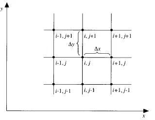
So, assuming initial conditons at time t=0 are known. For obtaining flow field variables at each grid point at next time step,
`f_(i,j)^(t+dt) = f_(i,j)^t + ((delf)/(delt))_(avg)*dt` ---> (22)
where f is any flow field variable
For example, let us consider density.
Eq. (22) becomes
`rho_(i,j)^(t+dt) = rho_(i,j)^t + ((delrho)/(delt))_(avg)*dt` ---> (23)
The average term in above equation is obtained by
`((delrho)/(delt))_(avg) = 0.5*(((delrho)/(delt))_((i,j),p)^t + ((delrho^*)/(delt))_((i,j),c)^t)` ---> (24)
where `((delrho)/(delt))_((i,j),p)^t` = rate of change of density obtained form predictor step
`((delrho^*)/(delt))_((i,j),c)^t` = rate of change of density obtained from corrector step
Predictor step:
In this step, the spatial terms in the governing equation are numerically discretized by forward differencing. Considering the continuity equation given by eq. (10), at time t,
`((delrho)/(delt))_((i,j),p) = -rho_i*(V(i+1)-V(i))/dx - rho_i**V_i*(lnA(i+1)-lnA(i))/dx-V_i*(rho(i+1)-rho(i))/dx`---> (25`
All the above flow field variables are non dimensional.
Next step in predictor step is to update the density value,
`rho^u = rho_(t-dt) + ((delrho)/(delt))_((i,j),p)*dt` ---> (26`
These steps are also implemented for momentum and energy equations.
Corrector step:
In this step, the governing equations are replaced with upadted values of flow field variables and then the spatial terms are numerically discretized by backward differencing.
Therefore, eq. (25) becomes
`((delrho^u)/(delt))_((i,j),c) = -rho_i^u*(V^u(i)-V^u(i-1))/dx - rho_i^u**V_i^u*(lnA(i)-lnA(i-1))/dx-V_i^u*(rho^u(i)-rho^u(i-1))/dx` ---> (27`
The above step is also implemented for momentum and energy equations.
Values of eq.(25) and (27) are substituted in eq. (24) to get `((delrho)/(delt))_(avg)`
Therefore, density at next time step will be
`rho_t = rho_(t-dt) + ((delrho)/(delt))_(avg)*dt` ---> (28)
The values of other flow field variables are obtained follwing the same steps.
This method is of second order accurate as forward differencing is done in predictor step and backward differencing in corrector step.
MATLAB Codes:
Three programs, one main program and two functions(one for non conservation form and other for conservation form) are written.
Main Program:
% Week 7 Challenge
% Mac Cormack method
% Main program

clear all
close all
clc

L = 3;
n = 31;
c = 0.5;
ts = 1400;
gamma = 1.4;
x = linspace(0,L,n);

% Non conservation form
[mflo_ncon,rho_ncon,v_ncon,t_ncon,mach_ncon,p_ncon] = maccormack_nonconservation(L,n,c,ts,gamma);

% Conservation form
[mflo_con,rho_con,v_con,t_con,mach_con,p_con,u1,u2,u3] = maccormack_conservation(L,n,c,ts,gamma);

figure(9)
aa = plot(x,mflo_ncon);
hold on;
bb = plot(x,mflo_con);
grid on;
legend([aa,bb],'mass flow rate - non conservation','mass flow rate - conservation');
xlabel('non dimensional length (x/L)');
ylabel('non dimensional mass flow rate ');
title('Comparison of Normalized mass flow rate distributions');

% Table

Form = {'Exact solution';'Non conservation';'Conservation'};
Normalized_density = [0.634;rho_ncon(round((n+1)/2));rho_con(round((n+1)/2))];
Normalized_temperature = [0.833;t_ncon(round((n+1)/2));t_con(round((n+1)/2))];
Normalized_pressure = [0.528;p_ncon(round((n+1)/2));p_con(round((n+1)/2))];
Mach_number = [1.000;mach_ncon(round((n+1)/2));mach_con(round((n+1)/2))];

throat = table(Form,Normalized_density,Normalized_temperature,Normalized_pressure,Mach_number)
The main program takes inputs such as length of domain, no. of grid points, no. of time steps and adiabatic index.
It plots a comparison graph of mass flow rates between conservation and nonconservation forms.
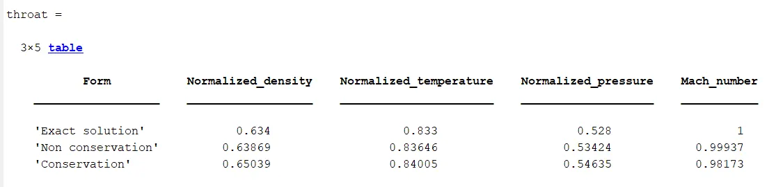
Also, a table is generated showing the values of primitive variables at middle of the domain. It is used for grid independence test.
Function for non conservation form:
% Week 7 Challenge
% function for Mac Cormack method
% f^(t+dt) = f^t + ((df/dt)_avg)^t*dt
% ((df/dt)_avg)^t = (df/dt)_p + (df*/dt)_c
% f*^t = f^t + (df/dt)_p*dt
% Non conservation

function [mflo_ncon,rho_ncon,v_ncon,t_ncon,mach_ncon,p_ncon] = maccormack_nonconservation(L,n,c,ts,gamma)

x = linspace(0,L,n);
dx = L/(n-1);

% initial condition at time t = 0
a = 1 + (2.2*((x-1.5).^2));
rho_ncon = 1 - (0.3146*x);
t_ncon = 1 - (0.2314*x);
v_ncon = (0.1 + 1.09*x).*(t_ncon.^0.5);
mflo_initial = rho_ncon.*a.*v_ncon;

nt = 1:ts;

time = 1;

% non conservation form of equations in dimesionless form

for k = nt

for j = 1:n
    ndt(j) = c*(dx/(t_ncon(j)^0.5 + v_ncon(j)));
end
    dt = min(ndt);

    rho_old=rho_ncon;
    v_old=v_ncon;
    t_old=t_ncon;

% Predictor step

for i = 2:(n-1)

    dvdx = (v_ncon(i+1)-v_ncon(i))/dx;
    dlogadx = (log(a(i+1))-log(a(i)))/dx;
    drhodx = (rho_ncon(i+1)-rho_ncon(i))/dx;
    dtdx = (t_ncon(i+1)-t_ncon(i))/dx;


% continuity
drhodt_p(i) = -rho_ncon(i)*dvdx - rho_ncon(i)*v_ncon(i)*dlogadx - v_ncon(i)*drhodx;

% momentum
dvdt_p(i) = -v_ncon(i)*dvdx - ((1/gamma)*(dtdx + ((t_ncon(i)/rho_ncon(i))*drhodx)));

%energy
dtdt_p(i) = -v_ncon(i)*dtdx - ((gamma-1)*t_ncon(i)*(dvdx + (v_ncon(i)*dlogadx)));

rho_ncon(i) = rho_ncon(i) + drhodt_p(i)*dt;
v_ncon(i) = v_ncon(i) + dvdt_p(i)*dt;
t_ncon(i) = t_ncon(i) + dtdt_p(i)*dt;

end

% corrector step

for q = 2:(n-1)

    dvdx = ((v_ncon(q)-v_ncon(q-1))/dx);
    dlogadx = (log(a(q))-log(a(q-1)))/dx;
    drhodx = (rho_ncon(q)-rho_ncon(q-1))/dx;
    dtdx = (t_ncon(q)-t_ncon(q-1))/dx;

% continuity
drhodt_c(q) = -rho_ncon(q)*dvdx - rho_ncon(q)*v_ncon(q)*dlogadx - v_ncon(q)*drhodx;

% momentum
dvdt_c(q) = -v_ncon(q)*dvdx - ((1/gamma)*(dtdx + ((t_ncon(q)/rho_ncon(q))*drhodx)));

%energy
dtdt_c(q) = -v_ncon(q)*dtdx - ((gamma-1)*t_ncon(q)*(dvdx + (v_ncon(q)*dlogadx)));

end

% average

drhodt = 0.5*(drhodt_p + drhodt_c);
dvdt = 0.5*(dvdt_p + dvdt_c);
dtdt = 0.5*(dtdt_p + dtdt_c);

% final solution update

for m = 2:(n-1)

rho_ncon(m) = rho_old(m) + drhodt(m)*dt;
v_ncon(m) = v_old(m) + dvdt(m)*dt;
t_ncon(m) = t_old(m) + dtdt(m)*dt;

% post processing Time-wise variation of the primitive variables
if (m == round((n-1)/2))
    rho_mid(k) = rho_ncon(m);
    v_mid(k) = v_ncon(m);
    t_mid(k) = t_ncon(m);
    p_mid(k) = rho_ncon(m)*t_ncon(m);
end

end

% Boundary conditions
% Inlet
v_ncon(1) = 2*v_ncon(2) - v_ncon(3);
rho_ncon(1) = 1;
t_ncon(1) = 1;
% Outlet
v_ncon(n) = 2*v_ncon(n-1) - v_ncon(n-2);
t_ncon(n) = 2*t_ncon(n-1) - t_ncon(n-2);
rho_ncon(n) = 2*rho_ncon(n-1) - rho_ncon(n-2);

mach_ncon = v_ncon./(t_ncon.^0.5);
p_ncon = rho_ncon.*t_ncon;
mflo_ncon = rho_ncon.*a.*v_ncon;

% Variation of Mass flow rate distribution inside the nozzle at different time steps during the time-marching process
if (time == 50)
    mflo_50 = rho_ncon.*a.*v_ncon;
end
if (time == 100)
    mflo_100 = rho_ncon.*a.*v_ncon;
end
if (time == 150)
    mflo_150 = rho_ncon.*a.*v_ncon;
end
if (time == 200)
    mflo_200 = rho_ncon.*a.*v_ncon;
end
if (time == 700)
    mflo_700 = rho_ncon.*a.*v_ncon;
end

time = time +1;
end


% Post processing
% Steady-state distribution of primitive variables inside the nozzle

figure(1)
subplot(5,1,1)
plot(x,v_ncon);
grid on;
xlabel('non dimensional length (x/L)');
ylabel('(v/a0)');
title('Variation of velocity wrt space - non conservation');
subplot(5,1,2)
plot(x,t_ncon);
grid on;
xlabel('non dimensional length (x/L)');
ylabel('(t/t0)');
title('Variation of temperature wrt space - non conservation');
subplot(5,1,3)
plot(x,rho_ncon);
grid on;
xlabel('non dimensional length (x/L)');
ylabel('(rho/rho0)');
title('Variation of density wrt space - non conservation');
subplot(5,1,4)
plot(x,p_ncon);
grid on;
xlabel('non dimensional length (x/L)');
ylabel('(p/p0)');
title('Variation of pressure wrt space - non conservation');
subplot(5,1,5)
plot(x,mach_ncon);
grid on;
xlabel('non dimensional length (x/L)');
ylabel('Mach no.');
title('Variation of mach number wrt space - non conservation');

figure(2)
plot(x,mflo_ncon);
grid on;
xlabel('non dimensional length');
ylabel('non dimensional mass flow rate');
title('Steady state mass flow rate distribution - non conservation');

% Timewise variation of primitive varibales
figure(3)
subplot(4,1,1)
plot(nt,rho_mid);
grid on;
xlabel('time');
ylabel('(rho/rho0)');
title('Timewise variation of density at throat - non conservation');
subplot(4,1,2)
plot(nt,v_mid);
grid on;
xlabel('time');
ylabel('(v/a0)');
title('Timewise variation of velocity at throat - non conservation');
subplot(4,1,3)
plot(nt,t_mid);
grid on;
xlabel('time');
ylabel('(t/t0)');
title('Timewise variation of temperature at throat - non conservation');
subplot(4,1,4)
plot(nt,p_mid);
grid on;
xlabel('time');
ylabel('(p/p0)');
title('Timewise variation of pressure at throat - non conservation');

% Variation of Mass flow rate distribution inside the nozzle at different time steps during the time-marching process
figure(4)
uu = plot(x,mflo_initial);
hold on;
vv = plot(x,mflo_50);
ww = plot(x,mflo_100);
xx = plot(x,mflo_150);
yy = plot(x,mflo_200);
zz = plot(x,mflo_700);
grid on;
legend([uu,vv,ww,xx,yy,zz],'at t = 0','at t = 50','at t = 100','at t = 150','at t = 200','at t = 700');
xlabel('non dimensional length');
ylabel('non dimensional mass flow rate');
title('Variation of mass flow rate distribution - non conservation');

end
This function calculates the values of primitive variables in the non conservation form of governing equations. It is iterated for various time steps which is given as input.
Plots are generated to show the steady state distribution of primitive variables, mass flow rate inside the nozzle, timewise variation of primitive variables at centre point of the domain and mass flow rate distribution at different time steps.
Function for conservation form:
% Week 7 Challenge
% function for Mac Cormack method
% f^(t+dt) = f^t + ((df/dt)_avg)^t*dt
% ((df/dt)_avg)^t = (df/dt)_p + (df*/dt)_c
% f*^t = f^t + (df/dt)_p*dt
% conservation

function [mflo_con,rho_con,v_con,t_con,mach_con,p_con,u1,u2,u3] = maccormack_conservation(L,n,c,ts,gamma)

x = linspace(0,L,n);
dx = L/(n-1);

% initial conditions at t = 0
for i = 1:length(x)

if (x(i) <= 0.5)
    rho_con(i) = 1;
    t_con(i) = 1;
else if (x(i) > 0.5 && x(i)<= 1.5)
        rho_con(i) = 1 - 0.366*(x(i)-0.5);
        t_con(i) = 1 - 0.167*(x(i)-0.5);
    else
        rho_con(i) = 0.634 - 0.3879*(x(i)-1.5);
        t_con(i) = 0.833 - 0.3507*(x(i)-1.5);
    end
end
a(i) = 1 + (2.2*((x(i)-1.5)^2));
v_con(i) = 0.59/(rho_con(i)*a(i));
e(i) = t_con(i);

u1(i) = rho_con(i)*a(i);
u2(i) = rho_con(i)*a(i)*v_con(i);
u3(i) = rho_con(i)*a(i)*((e(i)/(gamma-1) + (gamma/2)*v_con(i)^2));
f1(i) = u2(i);
uf(i) = (u2(i)^2)/u1(i);
f2(i) = uf(i) + (((gamma-1)/(gamma))*(u3(i)-((gamma/2)*uf(i))));
ug(i) = (u2(i)^3)/(u1(i)^2);
uk(i) = u2(i)*u3(i)/u1(i);
f3(i) = (gamma*uk(i)) - ((gamma*(gamma-1)/2)*ug(i));
% j(i) = ((gamma-1)/(gamma))*(u3(i)-((gamma/2)*uf(i)));
j(i) = (1/gamma)*rho_con(i)*t_con(i);
end

mflo_initial = rho_con.*a.*v_con;
nt = 1:ts;

time = 1;

% conservation form of equations in dimesionless form

for k = nt

for q = 1:n
    ndt(q) = c*(dx/(t_con(q)^0.5 + v_con(q)));
end
    dt = min(ndt);

    u1_old=u1;
    u2_old=u2;
    u3_old=u3;

% predictor

for w = 2:(n-1)

du1dt_p(w) = -(f1(w+1)-f1(w))/dx;

du2dt_p(w) = -(f2(w+1)-f2(w))/dx + (j(w)*(a(w+1)-a(w))/dx);

du3dt_p(w) = -(f3(w+1)-f3(w))/dx;

%solution update

u1(w) = u1(w) + du1dt_p(w)*dt;
u2(w) = u2(w) + du2dt_p(w)*dt;
u3(w) = u3(w) + du3dt_p(w)*dt;

rho_con(w) =u1(w)/a(w);
v_con(w) = u2(w)/u1(w);
t_con(w) = (gamma-1)*((u3(w)/u1(w))-(gamma*(v_con(w)^2)/2));

f1(w) = u2(w);
uf(w) = (u2(w)^2)/u1(w);
f2(w) = uf(w) + (((gamma-1)/(gamma))*(u3(w)-((gamma/2)*uf(w))));
ug(w) = (u2(w)^3)/(u1(w)^2);
uk(w) = u2(w)*u3(w)/u1(w);
f3(w) = (gamma*uk(w)) - ((gamma*(gamma-1)/2)*ug(w));
% j(w) = ((gamma-1)/(gamma))*(u3(w)-((gamma/2)*uf(w)));
j(w) = (1/gamma)*rho_con(w)*t_con(w);

% corrector

du1dt_c(w) = -(f1(w)-f1(w-1))/dx;

du2dt_c(w) = -(f2(w)-f2(w-1))/dx + (j(w)*((a(w)-a(w-1))/dx));

du3dt_c(w) = -(f3(w)-f3(w-1))/dx;

end

% average
du1dt = 0.5*(du1dt_p + du1dt_c);
du2dt = 0.5*(du2dt_p + du2dt_c);
du3dt = 0.5*(du3dt_p + du3dt_c);

% final solution update
for o = 2:(n-1)
    u1(o) = u1_old(o) + du1dt(o)*dt;
    u2(o) = u2_old(o) + du2dt(o)*dt;
    u3(o) = u3_old(o) + du3dt(o)*dt;
end

% Boundary conditions
% inlet
u1(1) = a(1);
u2(1) = 2*u2(2) - u2(3);
u3(1) = u1(1)*((t_con(1)/(gamma-1))+((gamma/2)*(v_con(1)^2)));
% outlet
u1(n) = 2*u1(n-1) - u1(n-2);
u2(n) = 2*u2(n-1) - u2(n-2);
u3(n) = 2*u3(n-1) - u3(n-2);

% primitive variables
for r = 1:n
    rho_con(r) =u1(r)/a(r);
    v_con(r) = u2(r)/u1(r);
    t_con(r) = (gamma-1)*((u3(r)/u1(r))-(gamma*(v_con(r)^2)/2));
    j(r) = (1/gamma)*rho_con(r)*t_con(r);

% post processing Time-wise variation of the primitive variables
if (r == round((n-1)/2))
    rho_mid(k) = rho_con(r);
    v_mid(k) = v_con(r);
    t_mid(k) = t_con(r);
    p_mid(k) = rho_con(r)*t_con(r);
end

end

% Updating flux vectors f and source term j
for y = 1:n
f1(y) = u2(y);
uf(y) = (u2(y)^2)/u1(y);
f2(y) = uf(y) + (((gamma-1)/(gamma))*(u3(y)-((gamma/2)*uf(y))));
ug(y) = (u2(y)^3)/(u1(y)^2);
uk(y) = u2(y)*u3(y)/u1(y);
f3(y) = (gamma*uk(y)) - ((gamma*(gamma-1)/2)*ug(y));
% j(y) = ((gamma-1)/(gamma))*(u3(y)-((gamma/2)*uf(y)));
end

mach_con = v_con./(t_con.^0.5);
p_con = rho_con.*t_con;
mflo_con = rho_con.*a.*v_con;

% Variation of Mass flow rate distribution inside the nozzle at different time steps during the time-marching process
if (time == 50)
    mflo_50 = rho_con.*a.*v_con;
end
if (time == 100)
    mflo_100 = rho_con.*a.*v_con;
end
if (time == 150)
    mflo_150 = rho_con.*a.*v_con;
end
if (time == 200)
    mflo_200 = rho_con.*a.*v_con;
end
if (time == 700)
    mflo_700 = rho_con.*a.*v_con;
end

time = time +1;
end

% Post processing
% Steady-state distribution of primitive variables inside the nozzle
figure(5)
subplot(5,1,1)
plot(x,v_con);
grid on;
xlabel('non dimensional length (x/L)');
ylabel('(v/a0)');
title('Variation of velocity wrt space - conservation');
subplot(5,1,2)
plot(x,t_con);
grid on;
xlabel('non dimensional length (x/L)');
ylabel('(t/t0)');
title('Variation of temperature wrt space - conservation');
subplot(5,1,3)
plot(x,rho_con);
grid on;
xlabel('non dimensional length (x/L)');
ylabel('(rho/rho0)');
title('Variation of density wrt space - conservation');
subplot(5,1,4)
plot(x,p_con);
grid on;
xlabel('non dimensional length (x/L)');
ylabel('(p/p0)');
title('Variation of pressure wrt space - conservation');
subplot(5,1,5)
plot(x,mach_con);
grid on;
xlabel('non dimensional length (x/L)');
ylabel('Mach no.');
title('Variation of mach number wrt space - conservation');

figure(6)
plot(x,mflo_con);
grid on;
xlabel('non dimensional length');
ylabel('non dimensional mass flow rate');
title('Steady state mass flow rate distribution - conservation');

% Timewise variation of primitive varibales
figure(7)
subplot(4,1,1)
plot(nt,rho_mid);
grid on;
xlabel('time');
ylabel('(rho/rho0)');
title('Timewise variation of density at throat - conservation');
subplot(4,1,2)
plot(nt,v_mid);
grid on;
xlabel('time');
ylabel('(v/a0)');
title('Timewise variation of velocity at throat - conservation');
subplot(4,1,3)
plot(nt,t_mid);
grid on;
xlabel('time');
ylabel('(t/t0)');
title('Timewise variation of temperature at throat - conservation');
subplot(4,1,4)
plot(nt,p_mid);
grid on;
xlabel('time');
ylabel('(p/p0)');
title('Timewise variation of pressure at throat - conservation');

% Variation of Mass flow rate distribution inside the nozzle at different time steps during the time-marching process
figure(8)
uu = plot(x,mflo_initial);
hold on;
vv = plot(x,mflo_50);
ww = plot(x,mflo_100);
xx = plot(x,mflo_150);
yy = plot(x,mflo_200);
zz = plot(x,mflo_700);
grid on;
legend([uu,vv,ww,xx,yy,zz],'at t = 0','at t = 50','at t = 100','at t = 150','at t = 200','at t = 700');
xlabel('non dimensional length');
ylabel('non dimensional mass flow rate');
title('Variation of mass flow rate distribution - conservation');

end
This function calculates the values of primitive variables in the conservation form of governing equations. It is iterated for various time steps which is given as input.
Plots are generated to show the steady state distribution of primitive variables, mass flow rate inside the nozzle, timewise variation of primitive variables at centre point of the domain and mass flow rate distribution at different time steps.
Outputs:
The inputs were given as length of domain(L) =3, no. of grid points(n) = 31, time steps(ts) = 1400, courant number (c) = 0.5, adiabatic index (gamma) = 1.4
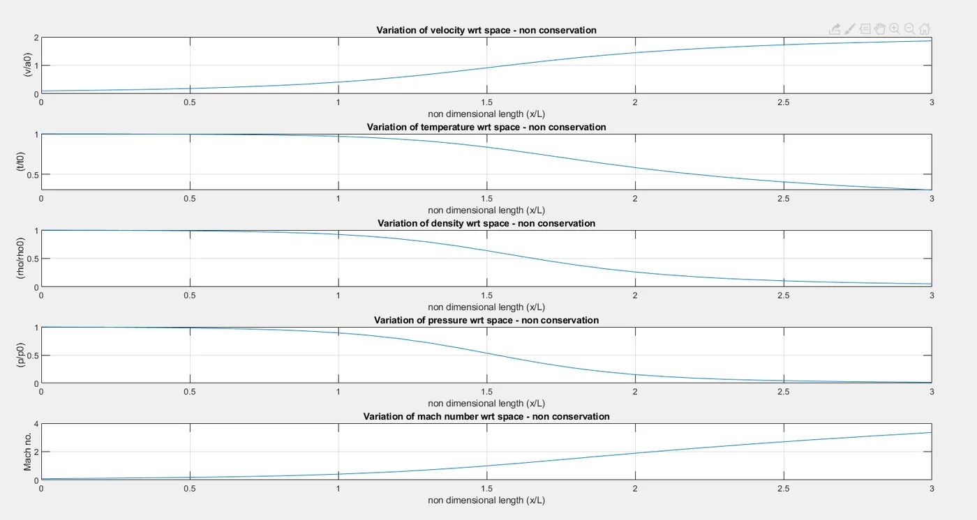
1. Non conservation form: (Figure 1)
(i) Steady-state distribution of primitive variables inside the nozzle:
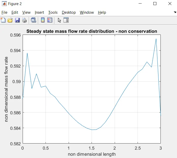
(ii) Mass flow rate: (Figure 2)
(iii) Timewise variation of primitive variables: (Figure 3)
(iv) Variation of Mass flow rate distribution inside the nozzle at different time steps during the time-marching process: (Figure 4)
2. Conservation form:
(i) Steady-state distribution of primitive variables inside the nozzle: (Figure 5)
(ii) Mass flow rate: (Figure 6)
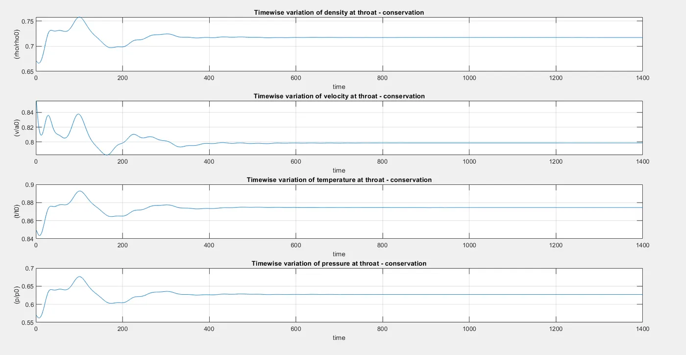
(iii) Timewise variation of primitive variables: (Figure 7)
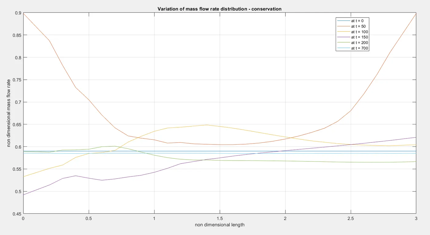
(iv) Variation of Mass flow rate distribution inside the nozzle at different time steps during the time-marching process: (Figure 8)
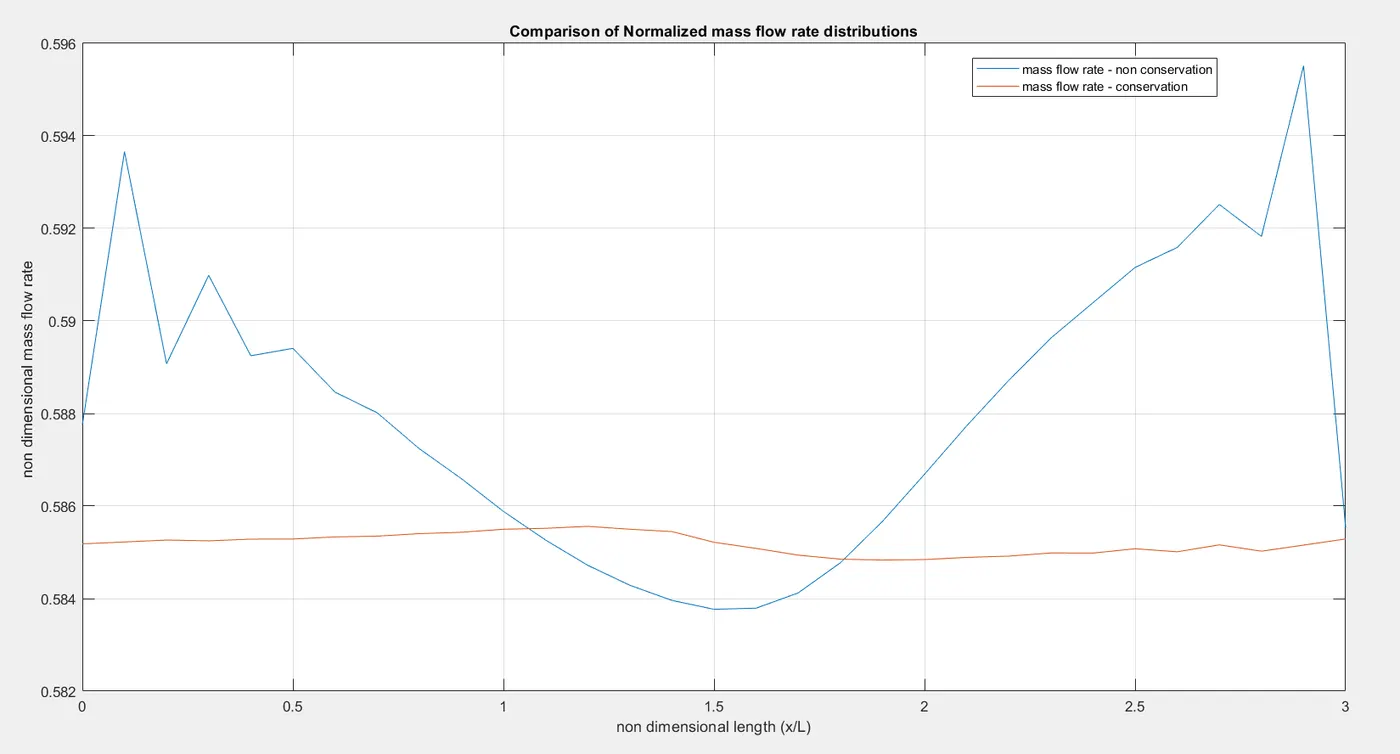
3. Comaprison of normalized mass flow rate distribution between conservation and non conservation forms: (Figure 9)
Conclusions:
1. For both conservation and non conservation forms,
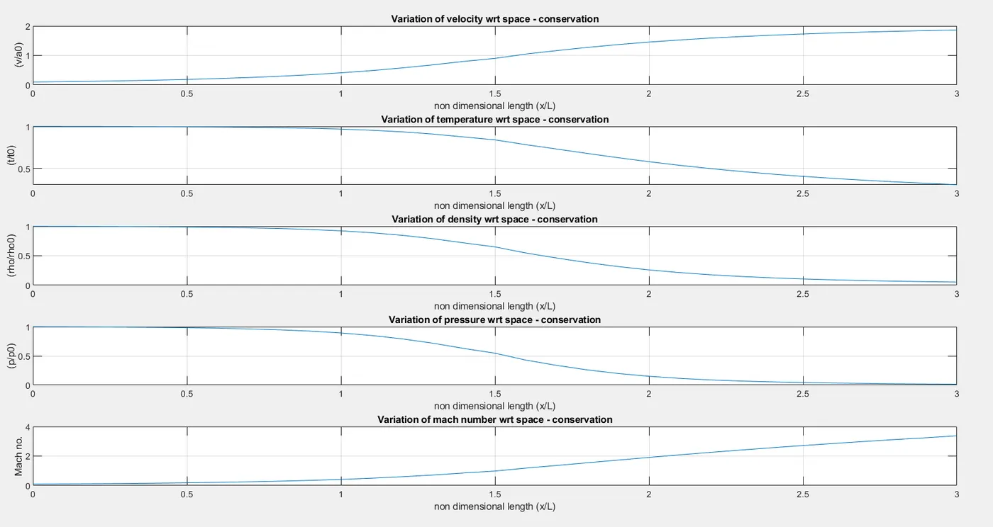
From figures (1) and (5), it is observed that the velocity and mach number increases from subsonic in the convergent section, sonic at the throat and supersonic in the divergent section. The temperature, pressure and density decreases with increase in length.
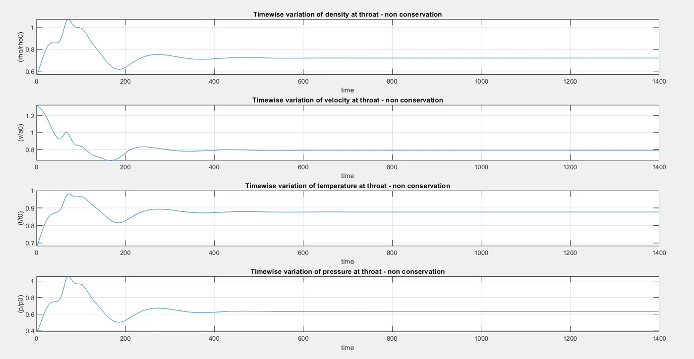
2. Figures (3) and (7) are plotted to observe the variation of flow field variables with time at throat(grid point 15).
For non conservation (Figure 3), it is observed that the density, temperature and pressure initially increases as time progresses and decreases suddenly upto 200th time step. There is considerbale amount of variation observed upto 200th time step. After this, the variation starts to reduce and becomes zero from 600th time step. The steady state is achieved after 600 time steps.
The velocity gradually decreases upto 200th time step and starts to increase and attains steady state after 600 time steps.
For conservation (Figure 7), similar to the non conservation, the density, temperature and pressure increases initially and suddeny decreases upto 200th time step but the variation is conseiderably less compared to non conservation. Steady state is attained after 600 time steps.
But the velocity behaviour is not same as non conservation. It fluctuates upto 200th time step and attains steady state after 600 time steps.
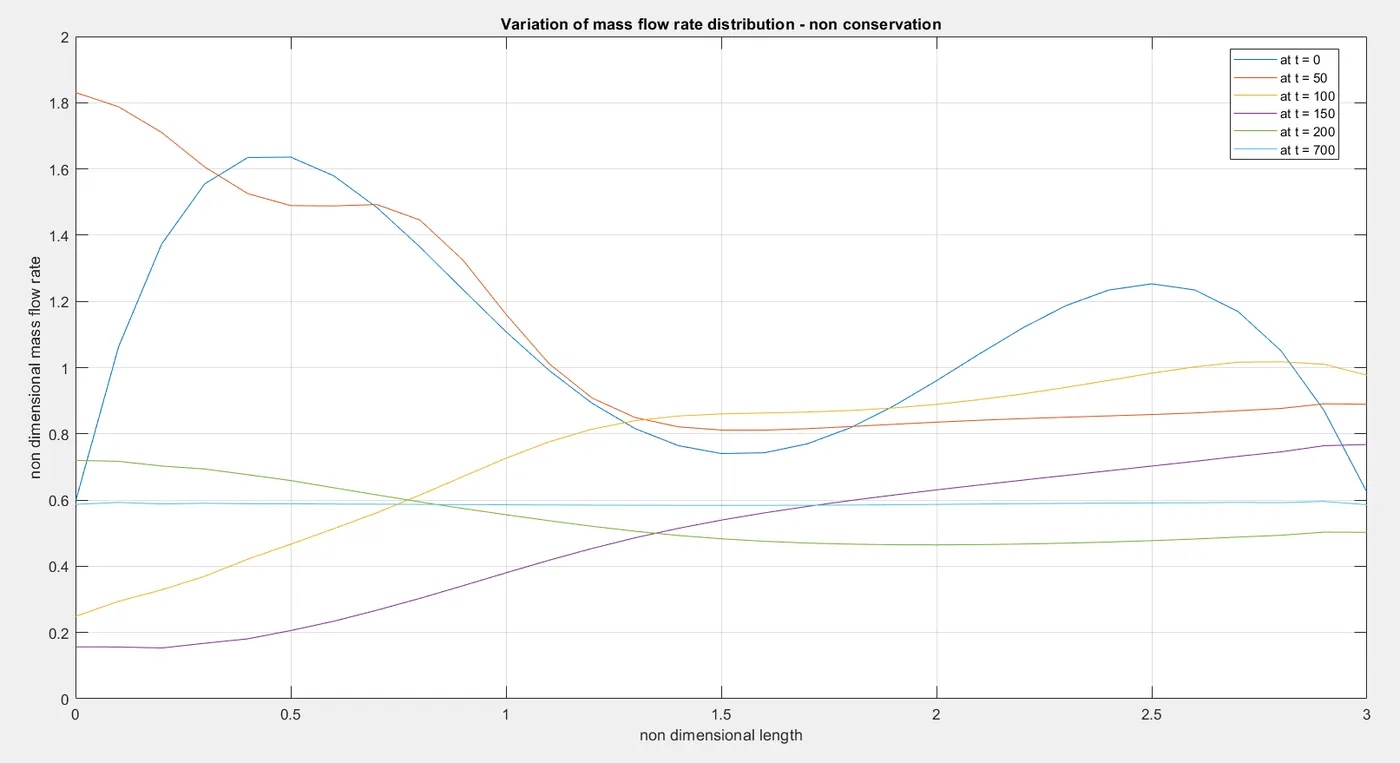
3. Figures (4) and (8) shows the normalized mass flow rate distribution during various time steps inside the nozzle.
For non conservation (Figure 4), the blue curve shows the mass flow distribution initially at time t = 0 (based on assumed initial conditions). After 50 time steps, the mass flow distribution has changed and after 100 time steps, it has changed radically. This is because the density and velocity have been varying rapidly at this stage and mass flow rate is directly proportional to velocity and density. After 200 time steps, the variation in mass flow rate is considerbaly decreased. After 700 time steps, mass flow rate curve is a staright line and has converged to a steady state value (approx. 0.58).
For conservation (Figure 8), the behaviour is similar to non conservation in which the mass flow rate varies rapidly upto 200 time steps, starts to settle down after 200 time steps and attains steady state after 700 time steps.
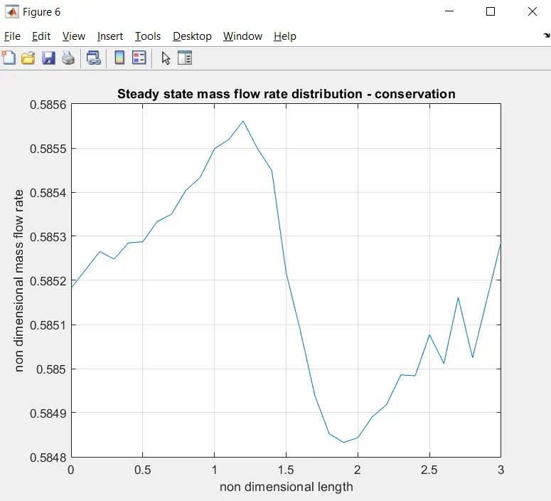
4. Figure 9 compares the mass flow distribution of conservation and non conservaion forms after steady state has been attained. It is observed that the variations of mass flow distribution in conservation form is much less than the variations observed in non conservation form.
The conservation for gives a dsitribution that is almost a constant whereas the distribution by non conservation form have more oscillations especially at both inflow and outflow boundaries.
It can be concluded that the conservation form preserves the mass flow better compared to non conservation form. This is because the mass flow rate is a dependent variable in conservation form of governing equations and is a primary result whereas the dependent variables in non conservation form are primitive variables and are obtained only after decoding the solution vector.
5. Grid Independence test:
As observed from previous studies, the solution might differ with incresase in no. of grid points. So, for a particular problem, if the solution (flow field variables) is found different with increase in grid points, it can be said that the solution is a function of no. of grid points. That particular solution cannot be considered final. To know whether a particular solution can be considered final or not, a grid independence must be done. In this, the no. of grid points are increased and the solution obtained is compared with the solution obtained form lesser grid points. If the difference is found out to considerbaly large, then again the no. of grid points are increased and the difference is found out. This process goes on until the difference becomes acceptable. Then it can be said that the solution reached grid independence and can be considered final.
For the above problem, the soluton is obtained for 31 grid points. A grid indpenedence test is perfomed by increasing the no. of grid points to 61 and both the solutions are compared to check whether the solution has reached grid independence or not.
Values of primitive variables at throat section are compared.
For n = 31:
For n = 61:

From the above data, it is observed that the values obatined at n = 61 are slightly more closer to the exact values compared to values at n = 31. The diference is very less of the order around 10^-4. This can be considered negligible. So, the solution at n = 31 can be considered final and it has achieved grid independence.