Week 9 - FVM Literature Review

FVM- Finite Volume Method

FVM method is basically a three dimensional application of the FDM method. It is used to reduce non-linear/ linear partial differential equations to algebraic forms and can be used to solve it numerically. FVM has lots of advantages compared to FDM, which will be discussed towards the end of the assignment. Here we make use of the Gauss Divergence theorem to approximate the PDEs to algebraic equations , and that can be solved using numerical processes.

Detailed Explanation :

Here we use a 1D heat conduction equation to be solved using the FVM method.

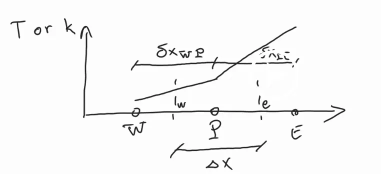
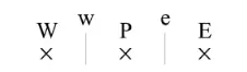
Consider the following figure:

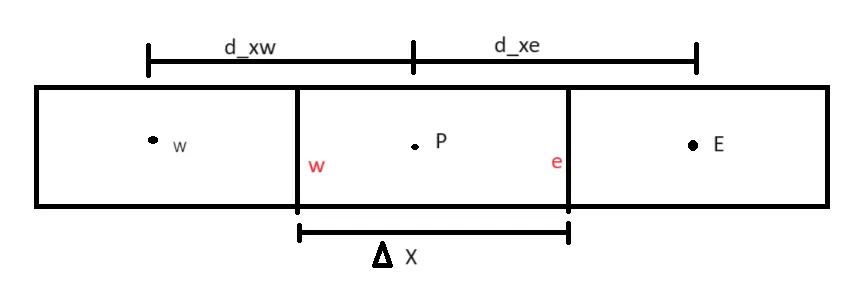
This is a uniform mesh with three elements. The size of each element is delta x and the distance between the nodes between the West W cell and the Present P cell is d_xw and d_xe for the one between P and E.

Consider the 1D steady state heat conduction equation :

The main essence of FVM method is the usage of gauss divergence theorem

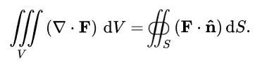
If you consider the 1D heat conduction equation, its given by

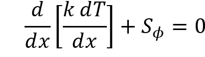
Intergrating this over a control volume, we get

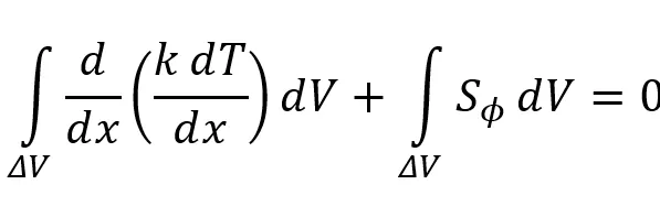
We apply the GD theorem and convert this volume integral to line integral( we check for the terms separately, starting with the diffusion term)

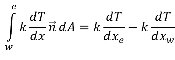
Here we assume unit volume, so A=1.

Now from the figure, we assume a linear profile to calculate the face values.

so the above equation becomes:

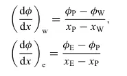
So the gradient terms becomes :

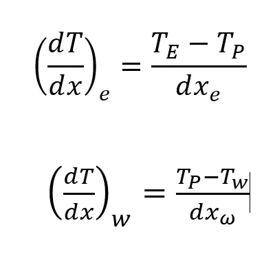
Here we assume the length of the mesh be equal to the distance between the nodes.

Substituting this in the final equation, we get

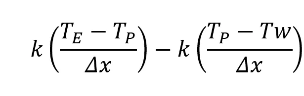
Here dx_e=dx_w=delta(x)

Now coming to the source term ,

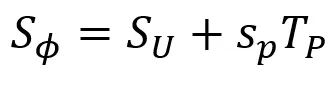
Phi here is the temperature (T). So we rewrite the whole equation

This is of the form (net heat flux in)-(net heat flux out)+ Source term =0

Now this particular equation is solved for every point in the domain and that is how FVM works

---

MAJOR DIFFERENCES BETWEEN FVM AND FDM

ASPECT	FVM(Finite Volume)	FDM(Finite Difference)
Mathematical Basis	Integral form of the conservation laws	Differential form of the governing equations
Discretization	Control volume based integration	Grid based approximation using Taylor series
Conservation	Locally conservative	Globally conservative
Geometry handling	Handles complex geometries and unstructured meshes	Best Suited for simple and structured grids
Accuracy & Stability	Robust and stable for flux conservation	High accuracy with potential stability issues
Implementation	Complex due to flux computation and irregular geometries	Simpler with regular grids
Applications	CFD, fluid flow, heat transfer	Heat conduction, wave propagation, etc.

---

INTERPOLATION SCHEMES

Consider the given node arrangement

We have the general transport equation which is given by :

When we just consider the case of 1D steady state convection diffusion, the equation becomes

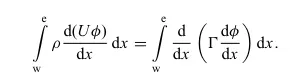
Converting this into algebraic form, we get :

Now the essence of face interpolation schemes come from how we calculate the face values from the nodal values

1. Central differencing

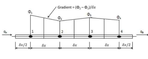
When it comes to linear interpolation , the averages of the nodal values are taken for the face values, and for the gradients. the following equations are used

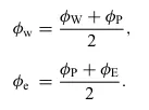
The figure below shows the central differencing in a graph :

This has certain advantages and disadvantages:

Advantages:

• Central differencing schemes offer second-order accuracy, meaning the error decreases quadratically as the grid spacing is reduced. This makes them significantly more accurate than first-order schemes for smooth functions.
  
• They introduce minimal numerical dispersion, which helps in maintaining the physical fidelity of solutions, particularly in wave propagation problems, making them ideal for smooth, continuous fields.
  

Disadvantages

• Cannot be used when the flow has high convection
• It cannot capture sharp gradients like shocks.

2. Upwind Scheme

To understand upwind schemes, we introduce a concept called the Peclet number. This is the ratio between convective mass transfer and diffusive mass transfer.

Given by the formula :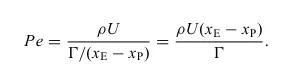

when you examine this from the final form of the equation given by :

you see that its the ratio of the convective term and diffusive term and if this Peclet number is very high, it means that the flow is highly convective. In this situation, you cannot use a central differencing scheme. Instead of taking the mere average of both the cell values, we need to account for the transportiveness of the flow. So we require another approach. Here we use the upwind schemes. Schemes that let face values be dependent only on upstream conditions are called upwind schemes.

Here what we assume is that the face values between two cells is the given the value of the nearest upstream cell. So if the flow is from west to east

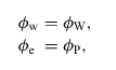
And if the flow is from east to west

So we substitute that in this and we get

But upwind schemes can have certain disadvantages :

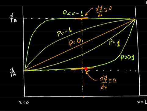
The disadvantage is that it overestimates the diffusion using a line phi - x relationship. To understand it further, consider the graph

( graph is taken from a Youtube video)

Here when Peclet number is much greater than 1, you see that the slope is almost 0, which is the diffusion. But upwind scheme still calculates this and over estimates the value. So we need other kinds if schemes for this.

3. QUICK Scheme

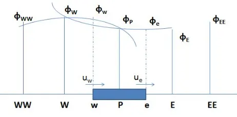
QUICK stands for Quadratic Upstream Interpolation for Convective Kinematics. This scheme is 3rd order accurate. This scheme is 3 point upstream weighted average scheme. The scheme takes two upstream values and one downstream values. In the aove figure, if the flow is going from left to right, if u>0, the phi _w is a function of phi_ww, phi_w and phi p and phi_e is a function of phi_w, phi_p and phi_e.

Here , phi is of the form Ax^2+Bx+C, when you solve the equation , you get :

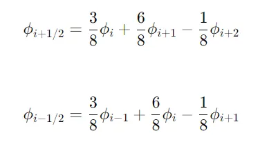
These are the main schemes used to calculate the face values, but there are other complex schemes too like MUSCL(Monotonic upstream centered scheme for conservation laws) and TVD Schemes etc.

---

FLUX LIMITERS

Flux limiters in computational fluid dynamic are mathematical tools used to control numerical fluxes in high-resolution schemes, ensuring a balance between accuracy and stability by preventing spurious oscillations near sharp gradients or discontinuities. They are usually used in high resolution schemes like MUSCL . Using flux limiters and high order schemes can make the solution TVD(Total Variation diminishing)