Week 3 - Solving second order ODEs

REPORT

AIM: Write a program in MatlabOctave that will simulate the pendulum motion

OBJECTIVE: 1.To create a plot of angular displacement and velocity with initial conditions

2.To create an animation of a pendulum as a function of time.

THEORY:

A simple pendulum is defined as a weight suspended from a massless string. Usually, it consists of a sphere with a mass 'm' which is suspended from a string whose mass is negligible compared to the sphere.

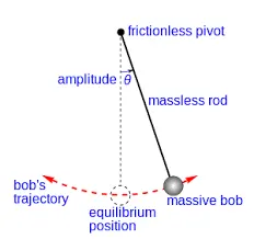
The given figure shows the terminologies of a pendulum aparatus.

SECOND ORDER ODE

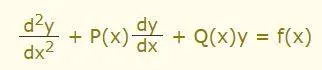
This is an example of a second-order ODE where the highest power is 2. The pendulum can be modeled into a second-order differential equation and this equation can be solved using Matlab.

If the order of an ODE is m, then Matlab breaks down this ODE to 'm' number of single ODES and it is solved using ODE45 solver which is an inbuilt Matlab solver that solves ODEs of the first order.

The theory behind the pendulum is given:

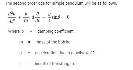
CALCULATIONS

let x=theta

now:

x=x1

so dx/dt=dx1/dt

dx1/dt=x2

so : d^2(x)/dt^2=d^2(x1)/dt^2=dx2/dt

substituting in the main equation , you get

dx2/dt+b/m*x2+g/L*sin(x1)

So writing in the matrix format:

d/dt[x1;x2]=[x2;-b/m*(x2)-g/L*sin(x1))]

CODE

close all
clear all
clc


theta_t=[0;5]; %initial conditions

time_span=linspace(0,10,500) %the time intervals where the values will be calculated

[t,results]=ode45(@(t,theta) ode_2(t,theta),time_span,theta_t)

plot(t,results(:,1))
hold on
plot(t,results(:,2))
xlabel('time')
ylabel('plot')
legend('displacement','velocity')

x=results(:,1)
ct=1

for i=1:length(x)
    t=x(i)
    x0=0
    y0=0
    x1=-(1*cos(90-t))
    y1=-(1*sin(90-t))
    
    figure(2)
    plot([-1 1],[0 0],"color",'k',"linewidth",4)
    hold on
    plot([x0 x1], [y0 y1],'linewidth',3)
    plot(x1,y1,'o','markers',10)
    hold off
    grid on
    axis([-2 2 -2 2])
    pause(0.04)
    M(ct)=getframe(gcf)
    ct=ct+1
    
end
movie(M)
videofile=VideoWriter('Pendulum.avi','Motion JPEG AVI');
open(videofile)
writeVideo(videofile,M)




function [ode]=ode_2(t,theta)

b=0.05;
g=9.81;
l=1;
m=0.1;
theta_1=theta(1) 
theta_2=theta(2) 


d_theta_1=theta_2
d_theta_2=-(b/m)*theta_2-(g/l)*sin(theta_1)

ode=[d_theta_1;d_theta_2]

link TO VIDEO:https://youtu.be/qxm3rj6FERg

OUTPUT GRAPHS

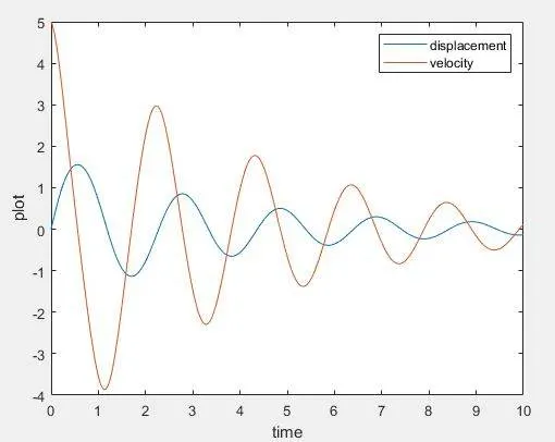
the given graph shows how the angular displacement and angular velocity is varying WRT to time .

STEPWISE CODE EXPLANATION

1. The initial angular velocity and displacement are given in the PGM
2. The linspace command is used to tell Matlab how theta is being varied
3. The ODE45 solver is used to solve the first-order differential equation
4. The '@' symbol is used for the anonymous function
5. The ode45 solver inputs the time span, initial condition, and a function where two parameters t and theta are passed
6. The function computes the value of theta_1 and theta_2 and is stored in an array.
7. theta_1 and theta_2 are found for all values of time and is stored in results
8. The graph is plotted
9. The loop is used to show how the pendulum is moving wrt to time.
10. The loop is set from 1 to length of results
11. The movement of the pendulum is analyzed using plot commands and the whole animation is made into a movie.

ERRORS FACED DURING PROGRAMMING

1. Make sure that the format of Ode45 solver is maintained. If else it will show an error similar to

2.Dont put Ct value as 0

CONCLUSION:

The graph has been plotted and animation has been created. The graph appears to be sinusoidal in nature.