Week 4 - Genetic Algorithm
PROJECT REPORT
AIM: Write a Matlab code to optimize the Stalagamite function and find the local maxima.
OBJECTIVE: 1.To understand the working of a genetic algorithm.
2. To form the Stalagamite expression.
3.To plot for unbounded and unconstrained conditions.
THEORY:
A genetic algorithm is a search heuristic that is inspired by Charles Darwin’s theory of natural evolution. This algorithm reflects the process of natural selection where the fittest individuals are selected for reproduction in order to produce offspring of the next generation.
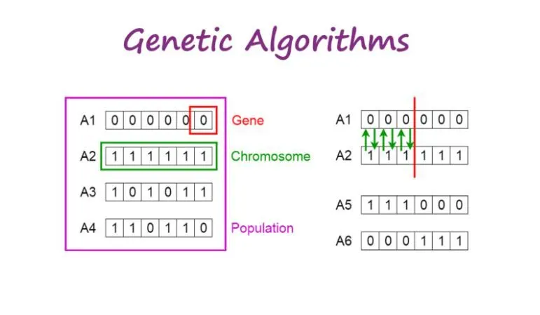
The process of natural selection starts with the selection of the fittest individual from a given population. They reproduce and have the traits and characteristics of their parents. If parents have good fits, their off-springs will have a better fit and will be more adapted to the environment. This process keeps on happening until the fittest generation is produced.
5 Phases are considered in the Genetic Algorithm:
- Initial population
- Fitness function
- Selection
- Crossover
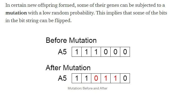
- Mutation
INITIAL POPULATION:
The process begins with a set of individuals which is called a Population. Each individual is a solution to the problem you want to solve. An individual is characterized by a set of parameters (variables) known as Genes. Genes are joined into a string to form a Chromosome (solution). In GA, binary strings are used to represent the genes of an individual parent.
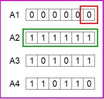
FITNESS FUNCTION
Fitness function is used to evaluate how fit the individual is. It gives a fitness score. The chances of an individual getting selected is based on fitness score
SELECTION
The selection phase is the phase where the fittest individual is selected and the genes are passes on to the off-springs
CROSSOVER
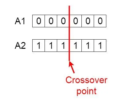
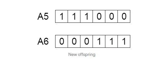
This is the most crucial phase. A cross over point is selected within the genes of the parents who are going to produce the off-springs. The genes are then crossed.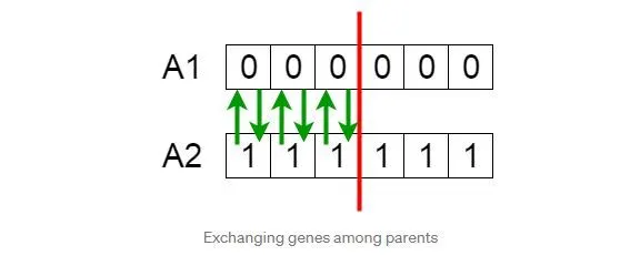
Now once this is done, new off-springs are added.
MUTATION
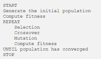
Pseudo Code of Genetic Algorithm is given below:
Advantages and Limitations
Adv:
- does not require any derivative information
- is faster and more efficient than traditional methods
- optimizes both continuous and discrete functions and also multi-objective problems
- Has parallel capabilities
- Useful when search space is very large and has lots of parameters involved.
Dis:
- calculation of fitness values might be computationally expensive for some problems
- if not implemented properly, Ga may not converge to an optimal solution.
GENETIC ALGORITHM FUNCTION (ga)
Ga is an inbuilt Matlab function that is used in optimization problems. The syntax of the function is given below:

This is the basic syntax. But it differs according to the number of inputs.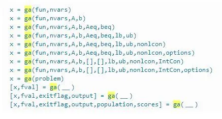
CODE
The code has 3 parts with one Stalgamite function. A Stalagmite mathematical model is used to obtain local maxima or minima. The equations are given below:
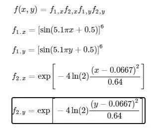
The code is given below:
1.Unbounded Inputs
clear all
close all
clc

x=linspace(0,0.6,150)
y=linspace(0,0.6,150)

[xx,yy]=meshgrid(x,y) % creating 3d mesh

for i=1:length(xx)    %loop that calculates the optimum value
    for j=1:length(yy);
    stal(1)=xx(i,j);
    stal(2)=yy(i,j);
    f(i,j)=stalgamite_1(stal);

    end

end


surf(xx,yy,f) %plotting
shading interp

[x,fval]=ga(@stalgamite_1,2)
Stalagmite Function:
function [y]=stalgamite_1(stal)
a=stal(1)
b=stal(2)

f1_x=(sin(5.1*pi*a+0.5)).^6; %calculating f1_x
f1_y=(sin(5.1*pi*b+0.5)).^6; %calculating f1_y

x1=-4.*log(2)*((a-0.0667).^2)./0.64;
f2_x=exp(x1);                %calculating f2_x

y1=-4.*log(2)*((b-0.0667).^2)./0.64;
f2_y=exp(y1)                 %calculating f2_y
final_f=f1_x.*f1_y.*f2_x.*f2_y;
y=(final_f);
OUTPUT
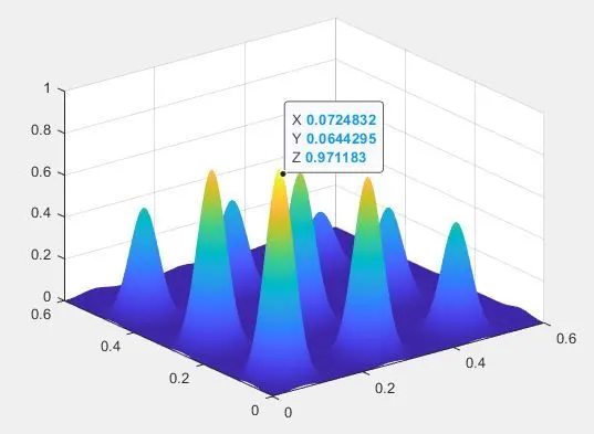
STEP BY STEP EXPLANATION OF CODE
- The given code is used to calculate the most optimized solution for the stalagmite function and find the local maxima.
- Initially, the search space is initialized. The 'linspace' command is used for this.
- Now the initialized x and y arrays are both converted into 3d arrays with the same number of rows and columns. 'Meshgrid' command is used for this.
- Now the x and y values are input using a nested for loop and the stalagmite function is obtained for all the values.
- Now 'surf' function is used to obtain the 3d plot
- Now the genetic algorithm is executed using the 'ga' command.
- In this command, the stalagmite function and the number of variables are given as the parameters and the most optimum value is obtained.
But this code has a fault because every time we execute the code, different values are obtained. This leads to ambiguity in solutions. This makes the code less reliable. The code given below shows this.
In the given below code, the stalagmite function is called for 50 times using a for loop and the statistical behaviour of the code is examined.
clc
clear ll
close all

x=linspace(0,0.6,150)
y=linspace(0,0.6,150)

[xx,yy]=meshgrid(x,y)


for i=1:length(xx)
    for j=1:length(yy)
        stal(1)=xx(i,j);
        stal(2)=yy(i,j);
        f(i,j)=call_stalagmite(stal);
    end
end

%surf(xx,yy,f)
%shading interp

for k=1:50
    [output,fval(k)]=ga(@call_stalagmite,2)
    x_opt(k)=output(1)
    y_opt(k)=output(2)

end

figure(1)
subplot(2,1,1)
hold on
surfc(x,y,f)
shading interp
plot3(x_opt,y_opt,fval,'marker','o','markersize',5,'markerfacecolor','r')
title('unbounded inputs')
subplot(2,1,2)
plot(fval)
xlabel('iterations')
ylabel('function min')
OBTAINED OUTPUT
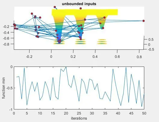
As it can be observed in the first plot, ga function plots different optimized values due to random sampling. In order to avoid this and for the solutions to converge, you can give the upper and lower bounds and also increase the population size. The code and outputs are given below:
1.Code and Output for the case with upper and lower bounds
clc
clear ll
close all

x=linspace(0,0.6,150)
y=linspace(0,0.6,150)

[xx,yy]=meshgrid(x,y)


for i=1:length(xx)
    for j=1:length(yy)
        stal(1)=xx(i,j);
        stal(2)=yy(i,j);
        f(i,j)=call_stalagmite(stal);
    end
end

%surf(xx,yy,f)
%shading interp
tic
for k=1:50
    [output,fval(k)]=ga(@call_stalagmite,2,[],[],[],[],[0;0],[1;1])
    x_opt(k)=output(1)
    y_opt(k)=output(2)

end

stud2_time=toc


figure(1)
subplot(2,1,1)
hold on
surfc(x,y,f)
shading interp
plot3(x_opt,y_opt,fval,'marker','o','markersize',5,'markerfacecolor','r')
title('unbounded inputs')
subplot(2,1,2)
plot(fval)
xlabel('iterations')
ylabel('function min')
This code follows the same steps as the previous code except that in the 'ga' command , the upper and lower bounds has been added and also subplot command is used to plot fval as a function of number of iterations and range.
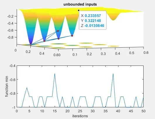
This plot gives a cleaner picture about the required point. This says that the required point is between the 6 peaks. In the second plot, the minimum value now falls between -0.4 and -1 which is much narrower range. This can further be optimized by increasing the population size. The code is give belowe:
%with increased population


clc
clear ll
close all

x=linspace(0,0.6,150)
y=linspace(0,0.6,150)

[xx,yy]=meshgrid(x,y)


for i=1:length(xx)
    for j=1:length(yy)
        stal(1)=xx(i,j);
        stal(2)=yy(i,j);
        f(i,j)=call_stalagmite(stal);
    end
end

%surf(xx,yy,f)
%shading interp
options=optimoptions('ga')
options=optimoptions(options,'populationsize',180)


tic
for k=1:50
    [output,fval(k)]=ga(@call_stalagmite,2,[],[],[],[],[0;0],[1;1],[],[],options)
    x_opt(k)=output(1)
    y_opt(k)=output(2)

end

stud2_time=toc


figure(1)
subplot(2,1,1)
hold on
surfc(x,y,f)
shading interp
plot3(x_opt,y_opt,fval,'marker','o','markersize',5,'markerfacecolor','r')
title('unbounded inputs')
subplot(2,1,2)
plot(fval)
xlabel('iterations')
ylabel('function min') 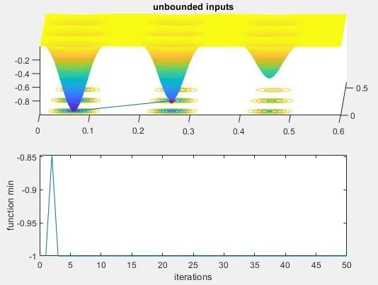
RESULT
It can be seen that as we give more constraints, the solution becomes more and more optimum. This is clearly evident from all the graphs.
The code has been developed, outputs obtained and studied.
ERRORRS FACED AND HOW TO RECTIFY
One many common error most people make is not passing the correct number of arguements in a functon.
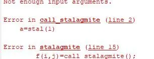
This can be avoided by making sure that right number of arguements are being passed.