Project 2 - Rankine cycle Simulator
PROJECT REPORT
AIM: The aim of the project is to simulate a Rankine cycle and plot the T-S and H-S graphs.
THEORY: The Rankine cycle is a model used to predict the performance of steam turbine systems. It was also used to study the performance of reciprocating steam engines. The Rankine cycle is an idealized thermodynamic cycle of a heat engine that converts heat into mechanical work while undergoing a phase change.
The ideal Rankine cycle consists of the following four processes, as shown in the T-s diagram :
1-2: Isentropic expansion in the turbine
2-3: Constant pressure heat rejection in the condenser
3-4: Isentropic compression in the pump
4-1: constant pressure heat addition in the boiler.
The figure is given below:
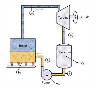
The steam expands isentropically in the turbine. It goes to the condensor where heat is rejected. The cold steam is taken to the pump where it is taken to the boiler and heat is added.
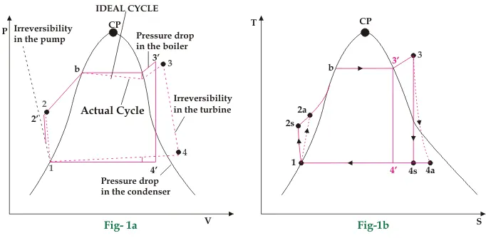
Mainly there are two plots:
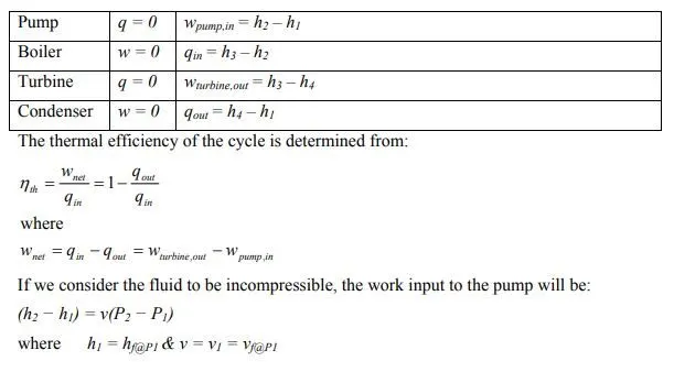
FORMULAS USED:
CODE
clear all
close all
clc

disp('                               RANIKINE CYCLE SIMULATOR                   ')
disp('1-2 Isentropic     compression    in         pump')
disp('2-3 constant pressure heat   addition in   boiler')
disp('3-4 isentropic expansion        in        turbine')
disp('4-1 constant pressure heat rejection in condensor')


%inputting p1,v1 and t1 values
disp('                              INPUTS                              ')
P_1=input('enter  pressure at turbine inlet (bars)                         : ');
T_1=input('enter the temperature  at turbine inlet (celcius)               : ');
P_2=input('enter the pressure at turbine outlet (bars)                     : '); %turbine outlet and condensor outlet are same
if (T_1==0):
    disp('cycle cannot be %f as inlet temp',T_1)

% calculating values at state point 1
P1=P_1;
T1=T_1;
H1=XSteam('h_pT',P1,T1);
S1=XSteam('s_pT',P1,T1);

%calculating values at state point 2
P2=P_2;
T2=T1*(P2/P1)^1.4;
S2=S1;
Sf2=Xsteam('sL_p',P2);
Sg2=XSteam('sV_p',P2);
X2=(S2-Sf2)/(Sg2-Sf2);
Hf2=XSteam('sL_p',P2);
Hg2=XSteam('sV_p',P2);
H2=Hf2+(X2*(Hg2-Hf2));

%calculating the values at state point 3

P3=P2;
T3=T2;
S3=XSteam('sL_p',P3,T3);
H3=XSteam('hL_p',P3,T3);

%calculating state points at 4
P4=P1;
%gamma=Cp/Cv,taking Cp and Cv from XSteam table
Cp=XSteam('CpL_p',P3);
Cv=XSteam('CvL_p',P3);
gamma=Cp/Cv;
g=(gamma-1)/gamma;
S4=S3;
T4=XSteam('T_ps',P4,S4);
H4=XSteam('h_pT',P4,T4);
S4_1=XSteam('sL_p',P4);
H4_1=XSteam('hL_p',P4);
S4_2=XSteam('sV_p',P4);
H4_2=XSteam('hV_p',P4);
T4_1=XSteam('T_hs',H4_1,S4_1);
T4_2=XSteam('T_hs',H4_2,S4_2);

%calculating the net work output and backwork ratio

Wt=H1-H2; %turbine work
Wp=H3-H4; %pump work
back_work_ratio=Wp/Wt; %backwork ratio
Wnet=Wt-Wp; %net work output
SSC=3600/Wt;

%data for plotting the graphs
t=linspace(0,500,600);

for i=1:length(t)
    sv(i)=XSteam('sV_T',t(i));
    sl(i)=XSteam('sL_T',t(i));
    hv(i)=XSteam('hV_T',t(i));
    hl(i)=XSteam('hL_T',t(i));
end


disp('                              RESULTS                     ')

disp('at state point 1 :')
fprintf('P1 is : %f bars \n',P1)
fprintf('T1 is : %f K \n',T1)
fprintf('H1 is : %f KJ \n',H1)
fprintf('S1 is : %f kg⋅m2⋅s−2⋅K−1 \n',S1)
fprintf('\n')

disp('at state point 2 :')
fprintf('P2 is : %f bars \n',P2)
fprintf('T2 is : %f K \n',T2)
fprintf('H2 is : %f KJ \n',H2)
fprintf('S2 is : %f kg⋅m2⋅s−2⋅K−1 \n',S2)
fprintf('X2 is : %f  \n',X2)
fprintf('\n')

disp('at state point 3 :')
fprintf('P3 is : %f bars \n',P3)
fprintf('T3 is : %f K \n',T3)
fprintf('H3 is : %f KJ \n',H3)
fprintf('S3 is : %f kg⋅m2⋅s−2⋅K−1 \n',S3)
fprintf('\n')

disp('at state point 4 :')
fprintf('P4 is : %f bars \n',P4)
fprintf('T4 is : %f K \n',T4)
fprintf('H4 is : %f KJ \n',H4)
fprintf('S4 is : %f kg⋅m2⋅s−2⋅K−1 \n',S4)
fprintf('\n')


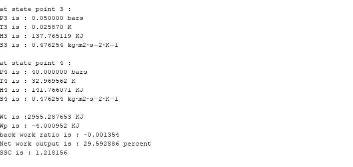
fprintf('Wt is :%f KJ \n',Wt)
fprintf('Wp is : %f KJ \n',Wp)
fprintf('back work ratio is : %f  \n',back_work_ratio)
fprintf('Net work output is : %f percent \n',Wnet/100)
fprintf('SSC is : %f \n',SSC)
fprintf('\n')


%plotting graphs for entropy and temperature

figure(1)
hold on
plot([S1 S2],[T1 T2],'color','r','linewidth',2)
text(S1,T1,'1')
text(S2,T2,'2')
plot([S2 S3],[T2 T3],'color','b','linewidth',2)
text(S3,T3,'3')
plot([S3 S4],[T3 T4],'color','g','linewidth',2)
text(S4,T4,'4')
plot([S4 S4_1],[T4 T4_1],'color','y','linewidth',2)
text(S4_1,T4_1,'4_1')
plot([S4_1 S4_2],[T4_1 T4_2],'color','r','linewidth',2)
text(S4_2,T4_2,'4_2')
plot([S4_2 S1],[T4_2 T1],'color','b','linewidth',2)
plot(sv,t)
plot(sl,t)
xlabel('entropy [kg⋅m2⋅s−2⋅K−1 ]')
ylabel('temperature [K]')
title('T-S plot')
legend('1-2 isentropic expansion','2-3 constant pressure heat addition','3-4 isentropic compression','constant pressure heat rejection')

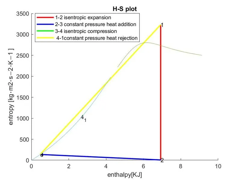
%plotting graphs for enthalpy and entropy

figure(2)
hold on
plot([S1 S2],[H1 H2],'color','r','linewidth',2)
text(S1,H1,'1')
text(S2,H2,'2')
plot([S2 S3],[H2 H3],'color','b','linewidth',2)
text(S3,H3,'3')
plot([S3 S4],[H3 H4],'color','g','linewidth',2)
text(S4,H4,'4')
plot([S4 S1],[H4 H1],'color','y','linewidth',2)
text(S4_1,H4_1,'4_1')
plot(sv,hv)
plot(sl,hl)
xlabel('enthalpy[KJ]')
ylabel('entropy [kg⋅m2⋅s−2⋅K−1 ]')
title('H-S plot')
legend('1-2 isentropic expansion','2-3 constant pressure heat addition','3-4 isentropic compression',' 4-1constant pressure heat rejection')
EXPLANATION OF THE CODE
- the code starts with inputting the initial turbine inlet and outlet pressure. The temperature is also given as input.
- The XSteam is an in-built Matlab steam table. After inputting the initial values, the enthalpy and entropy are calculated using the steam table.
- The values at state point 2 is obtained
- Since its isentropic process, you can use the formulas to calculate T2
- The Dryness factor (X) is calculated using the formula. For that Sf2 and Sg2 are found using the XSteam table.
- Now, Hf2 and Hg2 are found, and using the formula, enthalpy at state 2 is found.
- The entropy remains the same as from 1-2, its constant entropy.
- Similarly, state 3 and state 4 values are found.
- The turbine work, pump work, back work ratio, and net work output are calculated.
- The T-s and H-s figures are plotted.
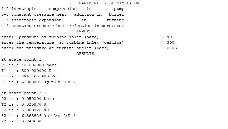
OUTPUT
PLOTS
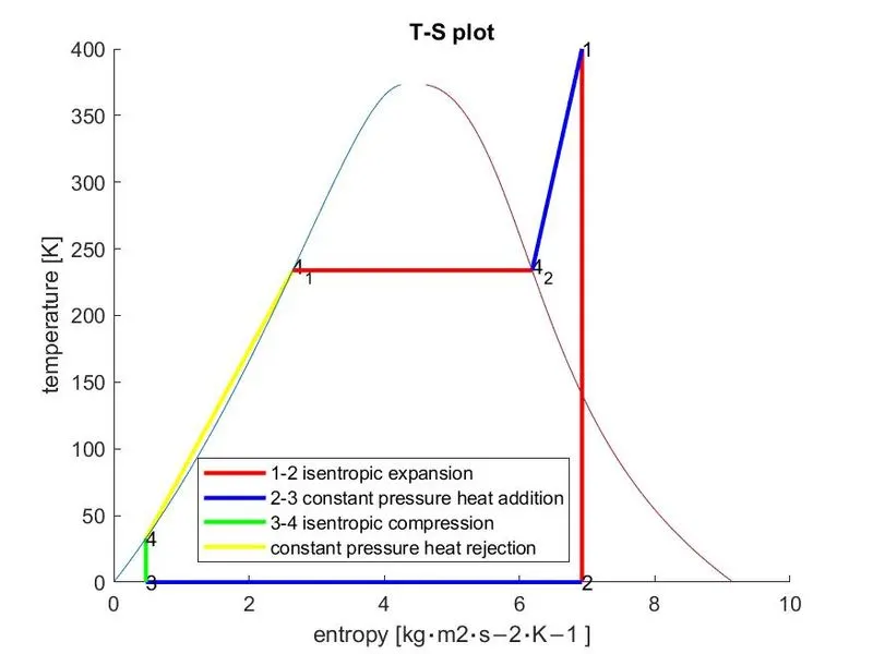
ERRORS OCCURED DURING PROGRAMMING
1. Make sure the same number of arguments are passed in the function.
2.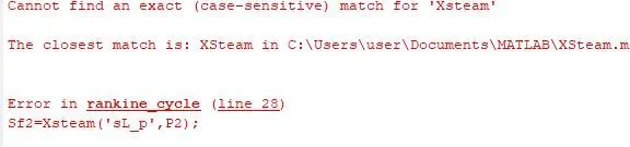
In this, XSteam should be written as it is, This command is case sensitive.
CONCLUSION
The code has been generated and run successfully and T-S and H-S graph has been plotted.