FVM Literature Review

⇒ What is Finite Volume Method?

 A discretization technique known as the finite volume method (FVM) is based on the integral form of the PDE that needs to be solved (such as the conservation of mass, momentum, or energy).

A finite volume (or cell) is provided, and the PDE is written in a form that can be solved for it. The governing equations are then solved for each finite volume in the discretized computational domain.]

 Flux calculation is crucial in FVM because the final system of equations frequently contains fluxes of the conserved variable. The primary benefit of this method over FDM is that it does not call for the use of structured grids. This means that the internal effort required to transform the provided mesh into a structured numerical grid is completely avoided.

 The approximate solution obtained is discrete, just like in FDM, but the variables are typically located at cell centers as opposed to nodal points. This isn't always the case because there are finite volume methods that are face-centered. In any case, interpolation is used to obtain the values of field variables at non-storage locations (for example, vertices)

Finite Difference Method	Finite Volume Method
1.  The Governing Equations are in differential form and the derived algebraic equations are solved as a results of discretization using Taylor Series Expansion	1. The Governing Equations are in integral form for a small control volume and the derived algebraic equations are solved as a result of approximation to the integration
2.  In FDM, it satisfies the governing equations in differential form	2. In FVM, it deals with the conservation of mass, momentum & energy equations
3. It uses the information only from the grid points for approximation of any function	3. It uses the average value from the cell for approximation of any function
4. In, FDM we need structured  grid mesh for performing analysis	4. In FVM, we dont need to bear the pain of structured mesh grids,
5. It is preferred for simulations with structured mesh grid	5. It is preferred and suitable for fluid flow simulations, heat transfer etc

 ⇒ Need For Interpolation Scheme & Flux Limiters in FVM

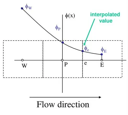
In Finite Volume Method(FVM) the flow variables are stored in the centroid of the cell

The Navier Stroke Equation is integrated across the cell volume i.e volume integrals are solved for each cell.The Navier Stroke Equation normally contains convection term,pressure gradient,diffusion term and a source term

For solving the convection & diffusion terms, the divergence theorem is used and the volume integrals are converted into surface integrals

Each cell can have number of faces depending on the type of mesh and each face will be associated with a neighbouring cell.

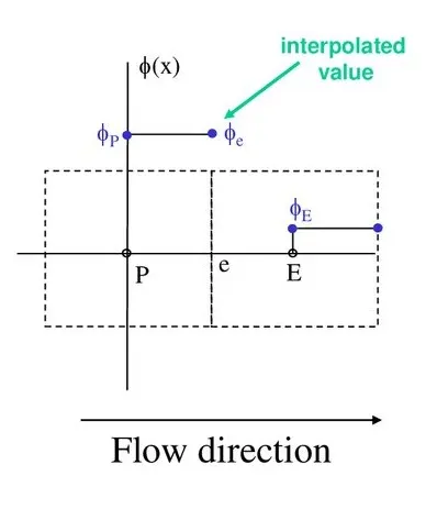
   First Order Upwind Scheme

• It is the simplest numerical scheme where we can assume the value at the face which is the same value as of the cell centered in the upstream face cell
• It is easy to implement and it provides stable results

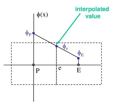
Central Differencing Scheme

• In this method the value of gradient is determined at the face by linear interpolation method between the cell centered values
• It is more accurate than first order upwind scheme, but it leads to oscillations in the solution or divergence if the Peclet Number is larger than 2.
• If the Pecelet Number is greater than 2, it is common to switch to first order upwind scheme..Such approach is also known as Hybrid Scheme

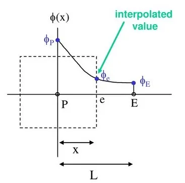
Power Scheme

• It is based on the analytical solution of the 1-D Convection-Diffusion Equation
• The face value is determined from an exponential profile through the cell values.
• If Pecelet Number is greater than 10, diffusion is ignored and first upwind method is used

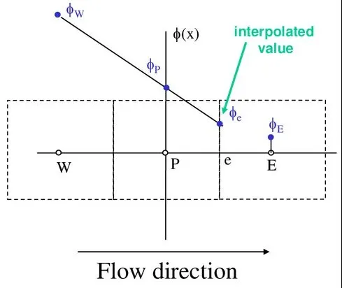
 Second Order Upwind Scheme

• In this method we need to determine the value of gradient from the cell values in the two cells upstream value at the face
• It is more accurate than the first order upwind scheme, but in regions with strong gradients it can result in face values that are outside of the range of cell values.
• It is one of the popular numerical schemes because of its accuracy and stability

Quick Scheme

• It stands for Quadratic Upwind Interpolation for Convection Kinetics.
• A quadratic curve is fitted  through two upstream nodes and one downstream node
• It is very accurate scheme but in regions of strong gradient, overshoot and undershoot can occur

Flux Limiters

The gradients tend to toggle, and they are also not bound to a particular value and keep oscillating. This oscillation occurs due to discontinuity due to shock.
Flux limiters help us rebound the gradient value and eventually help us reach a stable solution.
Numerical approximations use higher-order spatial discretization schemes, which results in better accuracy but exibits oscillations near discontinuities such as shocks. On the other hand, lower-order spatial discretization schemes remain stable near discontinuities but dampen out the distributions because of their dissipative nature.

Flux limiters operate as a functional switch and help in tuning the numerical fluxes obtained from the lower-order scheme and higher-order scheme, such that near the discontinuity the lower-order scheme is employed and away from it the higher-order scheme is employed.

1D Linear Heat Conduction To Demonstrate FVM 

(del/(delX))(alpha.(delT/(delX)) + S = 0.. eqn(1)

where S = Source Term ;  alpha = Diffusivity ;

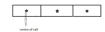
Here, we are taking  three control volumes, points inside each volume acts as the centre of the volume & PDE are solved for complete volume using the surface integral method i.e Gauss Divergence Method

Here in the above figure, the centre cell is denoted as P where as the east and west cells are denoted as E & W and small e & w acts as a junction between these cells.

At e & w interpolation schemes are used

int(del/(delX)(alpha.(delT)/(delX))dV+ intSdV = 0

int(del/(delX)(alpha.(delT)/(delX))Adx+ intSdV = 0

[(alphaAdelT)/(delx)] + int SdV =0

int S.dV = barS.dV

alphae [(AdelT)/(delXe )] - alphaw [(AdelT)/(delXw )] + barSdV = 0

alphaA[(Te - Tp)/(trianglex)] - alphaA[(Tp - Tw)/(trianglex)] + barS.dV = 0

Here we are finding an average which is denoted using S bar and when S bar is multiplied with dv this volume is equal to  the integral S.dv only

The integral sign is just getting replaced with average which is eventually the area under curve S.dV

Now, finally after integrating our main equation we get 

alphaA[(Te - Tp)/(trianglex)] - alphaA[(Tp - Tw)/(trianglex)] + Su + SpTp = 0 ... eqn ( 2)

as our final equation 

which is Heat Flux In - Heat Flux Out + Source Terms = 0

From the above equation 2, we can conclude that the FVM Methods are conservative in nature as the Total Heat Sum is equal to zero