Week 9 - FVM Literature Review

Week 9 - FVM Literature Review

AIM :

What is Finite Volume Method(FVM), write down the major differences between FDM & FVM. Also, describe the need for interpolation schemes and flux limiters in FVM.

You can use the 1D linear heat conduction equation as an example.

•Let us use the general transport equation as the starting point to explain the FVM, •We want to solve the general transport equation for the transported quantity in a givendomain, with given boundary conditions BC and initial conditions IC. •This is a second order equation. For good accuracy, it is necessary that the order of the discretization is equal or higher than the order of the equation that is being discretized. •By the way, starting from this equation we can write down the Navier-Stokes equations (NSE). So everything we are going to address also applies to the NSE

indicate several disadvantages associated with various discretization schemes for fluid flow simulations:

Finite Difference Method: It is difficult to satisfy conservation and to apply for irregular geometries

Finite Volume Method: It tends to be biased toward edges and one-dimensional physics.

Finite Element Method: It is difficult to solve hyperbolic equations using FEM.

Discontinuous Galerkin: It is the best (and worst) of all worlds.

Fluctuation Splitting: They are not yet widely applicable.

Finite Volume Method (FVM) is a numerical technique used for solving partial differential equations (PDEs), particularly in fluid dynamics and heat transfer problems. It discretizes the domain into small control volumes (or finite volumes) where the governing equations are integrated over each volume. FVM is a conservative method, meaning it ensures the conservation of quantities (e.g., mass, energy) within the control volumes.

Major Differences between FDM (Finite Difference Method) and FVM (Finite Volume Method):

1. Grid representation:

   • FDM discretizes the domain by dividing it into a grid of points, and the derivatives of the unknowns are approximated at these grid points.
   • FVM discretizes the domain by dividing it into control volumes (polygons in 2D or polyhedra in 3D). The unknowns are then averaged or integrated over these volumes.

2. Conservation:

   • FDM is not inherently conservative, which means that conservation properties of the underlying equations might not be preserved during the discretization process.
   • FVM is inherently conservative since it directly operates with control volumes, ensuring the conservation of quantities within each volume.

3. Treatment of boundaries:

   • In FDM, boundary conditions are often handled through explicit ghost cells or boundary nodes.
   • In FVM, boundary conditions are imposed by constructing appropriate fluxes at the control volume faces, considering the flow of quantities across the boundaries.

4. Geometrical flexibility:

   • FDM typically works well with structured grids, but handling complex geometries can be challenging.
   • FVM is more flexible in handling arbitrary geometries, especially unstructured grids, making it suitable for problems with complex boundaries.

Need for Interpolation Schemes and Flux Limiters in FVM:

In FVM, when integrating the governing equations over control volumes, we need to determine the values of variables at the faces of the control volumes. This requires interpolating values from the control volume centers to the faces.

Interpolation Schemes: Interpolation is necessary to approximate the values at the faces. Common interpolation schemes include piecewise constant, linear, quadratic, or higher-order interpolation. The choice of interpolation scheme affects the accuracy and stability of the FVM solution.

Flux Limiters: Flux limiters are used to prevent excessive oscillations, especially in high-contrast regions, such as shocks or discontinuities, that may arise during the numerical solution. These limiters restrict the magnitude of the numerical fluxes, ensuring stability and preventing unphysical solutions.

1D Linear Heat Conduction Equation Example:

Consider the 1D linear heat conduction equation:

∂u/∂t = α * ∂^2u/∂x^2

where u(x, t) is the temperature distribution, α is the thermal diffusivity, x is the spatial coordinate, and t is time.

Using FVM, the domain is divided into control volumes, and the heat conduction equation is integrated over each control volume. The interpolated values of u at the faces of the control volumes are used to construct the numerical fluxes. To ensure stability and accuracy, appropriate flux limiters are employed.

By solving the resulting system of algebraic equations for each control volume, the time-dependent temperature distribution u(x, t) can be obtained numerically throughout the domain.

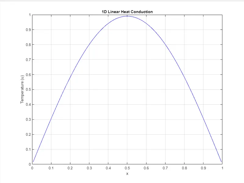
D Linear Heat Conduction Equation as MATLAB code:

As an example, let's consider the 1D linear heat conduction equation:

∂u/∂t = α * ∂²u/∂x²

where u is the temperature, t is time, x is the spatial coordinate, and α is the thermal diffusivity.

For simplicity, let's assume a uniform grid with spacing Δx and time step Δt. We'll use an explicit time-stepping scheme (Forward Euler) and a second-order central difference scheme for spatial discretization.

Example :

% 1D Linear Heat Conduction Equation Solver using FVM (Explicit)
clear; clc;

% Parameters
L = 1.0;          % Length of the domain
T_final = 0.1;    % Final simulation time
alpha = 0.01;     % Thermal diffusivity
Nx = 100;         % Number of spatial control volumes
Nt = 1000;        % Number of time steps

% Grid and initial condition
dx = L / Nx;
dt = T_final / Nt;
x = linspace(dx/2, L-dx/2, Nx);  % Cell center positions
u = sin(pi * x);                 % Initial temperature distribution

% Time-stepping loop
for t = 1:Nt
    u_new = u;
    for i = 2:Nx-1
        % Second-order central difference scheme
        d2u_dx2 = (u(i+1) - 2*u(i) + u(i-1)) / dx^2;
        
        % Update the solution using Forward Euler method
        u_new(i) = u(i) + alpha * dt * d2u_dx2;
    end
    u = u_new;
end

% Plot the final temperature distribution
plot(x, u, 'b-');
xlabel('x');
ylabel('Temperature (u)');
title('1D Linear Heat Conduction');
grid on;