Week 9 - FVM Literature Review

Objective: To study and understand

1. Finite Volume Method(FVM)
2. The difference between FDM and FVM
3. Interpolation schemes in FVM
4. Flux limiters in FVM

Description:

There are four numerical methods in total:

1. Finite Element Method (FEM)
2. Boundary Element Method (BEM)
3. Finite Volume Method (FVM)
4. Finite Difference Method (FDM)

FVM:

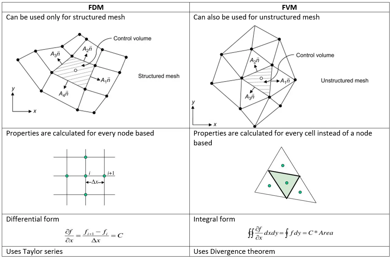
The finite-volume method is similar to the finite-differencing method in that the CAD model is first divided into very small but finite-sized elements of geometrically simple shapes. Apart from this, the finite-volume method is very different from the finite-differencing method, beginning with the concept of elements, which are instead referred to as cells.

A finite volume method (FVM) discretization is based upon an integral form of the PDE to be solved (e.g. conservation of mass, momentum, or energy) and can handle discontinuities in solutions. The PDE is written in a form which can be solved for a given finite volume (or cell). The computational domain is discretized into finite volumes and then for every volume the governing equations are solved. The resulting system of equations usually involves fluxes of the conserved variable, and thus the calculation of fluxes is very important in FVM.

The finite-volume method’s strength is that it only needs to do flux evaluation for the cell boundaries. This also holds for nonlinear problems, which makes it extra powerful for robust handling of (nonlinear) conservation laws appearing in transport problems.

The local accuracy of the finite-volume method, such as close to a corner of interest, can be increased by refining the mesh around that corner. However, the functions that approximate the solution when using the finite-volume method cannot be easily made of higher order. This is a disadvantage of the finite-volume method compared to the finite-difference method.

The basic advantage of this method over FDM is it does not require the use of structured grids, and the effort to convert the given mesh in to structured numerical grid internally is completely avoided. As with FDM, the resulting approximate solution is a discrete, but the variables are typically placed at cell centre’s rather than at nodal points. This is not always true, as there are also face-centered finite volume methods. In any case, the values of field variables at non-storage locations (e.g. vertices) are obtained using interpolation.

FVM can guarantee the local and global conservation of the system.

FDM

Boundary conditions are needed to truncate the computational domain. They represent communication with the surrounding world, which is the part that we do not want included in our simulation. With the finite-difference method, we may easily run into problems handling boundaries for the purpose of defining the boundary conditions.

The finite-difference method is the most direct approach to discretizing based upon the differential form of the PDE to be solved. We consider a point in space where we take the continuum representation of the equations and replace it with a set of discrete equations, called finite-difference equations.

The finite-difference method is typically defined on a regular/structured grid (i.e. the computational domain is usually divided into hexahedral cells (the grid), and the solution will be obtained at each nodal point.) and this fact can be used for very efficient solution methods. Regular grids are useful for very-large-scale simulations on supercomputers.

The method is therefore not usually used for irregular CAD geometries, but more often for rectangular or block-shaped models.

Examples include Formula 1 car computational-fluid-dynamic (CFD) simulations and space-shuttle CFD simulations. The finite-difference method is more difficult to use for handling material discontinuities. In addition, it does not lend itself for local grid refinement or anything similar to “adaptive mesh refinement.” This may be needed to resolve local rapid variations in solutions such as around a corner of a complex shape, as described earlier.

But, if we can fit the simulation in a rectangular or box-shaped geometry using a regular grid, efficient implementations are much easier than for finite-volume methods.

Interpolation schemes:

The approximations of surface and volume integrals require values of the variable at location other than the computational nodes of the control volume. Values at these locations are obtained using interpolation formulae.

Interpolation methods:

• Upwind interpolation
• Linear interpolation
• Quadratic upwind interpolation
• Hybrid, TVD and ENO interpolation schemes

Upwind interpolation (UDS)

This scheme takes into account the direction of fluid flow and based on it the value of solution variable at the face is approximated by its value at the upstream computational node. For example, if the fluid is moving from west to east, then:

`ϕ e ≈ ϕ P`

if the fluid is moving from east to west , then:

`ϕ e ≈ ϕ E`

This interpolation scheme is equivalent to using Forward difference method or backward difference method depending on the flow direction.

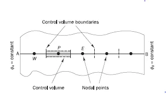
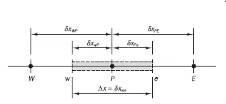
If the flow is along −X direction, then the values for this at the interface is given by

for`v > 0 ; u i − 1 2 ≈ u i − 1 ; u i + 1 2 ≈ u i`

`I c ≈ v (u i − u i − 1)/( Δ x)`which is equivalent to Backward Difference aScheme

Linear Interpolation Scheme:

In order to approximate the value of variable at control volume face center by two nearest computational nodes location e. This is equivalent to a central difference scheme of first order derivative. It is second order accurate and produce oscillatory solutions.

`f e = f E λ e + f p ( 1 − λ e )`

where `λ e = (x e − x p)/( x E − x P)`

Average interface values are given by

It is said to be equivalent because both these methods are of order of accuracy 2.

Advantages:

• Approximation of gradients has second order of accuracy on uniform grids
• Its formally of first order on non-uniform grids.

Disadvantages:

• It may produce oscillatory solutions in case of large grid space.

Hybrid interpolation scheme:

It is the blend of UDS and CDS. The hybrid difference scheme exploits the favourable properties of the
upwind and central differencing schemes. It switches to upwind differencing when central differencing produces inaccurate results at high Pe numbers.

The scheme is fully conservative and since the coefficients are always positive it is unconditionally bounded. It satisfies the transportiveness requirement by using an upwind formulation for large values of Peclet number.

`f e = γ f C D S + ( 1 − γ ) f U D S`

Advantages:

• Produces physically realistic solutions and highly stable compared to QUICK

Disadvantages:

• Accuracy is of first order.

Quadratic Upwind Interpolation for convective kinematics (QUICK):

It approximates the values of the variable at the CV face centre by Quadratic Interpolation of the values at three nearest computational nodes (1 Down stream node D & 2 Up stream nodes U , UU).

Quadratic - As it uses 3 nodes

Upwind - As it uses two upstreams

Convective Kinematics - As it is used for convective domain problems

Advantages:

• It is the better version of UDS and CDS because it is more accurate than UDS and more damping in nature than CDS as it uses 3 nodes to solve.
• It is of 3rd order accurate.

Disadvantages:

• The use of QUICK can lead to subtle problems caused by such unbounded results.
• Implementation of boundary conditions can be problematic with such higher-order schemes.

Total variation diminishing scheme (TVD):

The fact that the QUICK scheme and other higher-order schemes can give undershoots and overshoots has led to the development of second-order schemes that avoid these problems. The class of TVD (total variation diminishing) schemes has been specially formulated to achieve oscillation-free solutions and has proved to be useful in CFD calculations.

TVD schemes are designed to address this undesirable oscillatory behaviour of higher-order schemes. In TVD schemes the tendency towards oscillation is counteracted by adding an artificial diffusion fragment or by adding a weighting towards upstream contribution.

It is 2nd order accurate.

`f e = f p + 1/ 2 ψ ( r ) ( f E − f P )`

where,

ψ(r) is called a flux limiter function

Flux limiter:

For convective fluid flow, it is ovservedthat low order schemes are usually stable but quite dissipative in nature around the points of discontinuity or shocks while the higher order schemes are unstable in nature and show oscillations in the vicinity of dinscontinuity or shocks. Highly accurate and oscillation free schemes are known as High Resolution Schemes.

Flux Limiter functions are used to fine tune the higher order and lower order schemes in such a way that the resulting scheme gives a higher order accuracy in the smooth region of the flow and maintains first order accuracy in the vicinity of shocks and discontinuities. For such a scheme TVD scheme is employed.

where,

flow is low precision flux (first order)

fhigh is high precision flux (higher order)

Conlusion:

The Finite Volume Method (FVM) is a particularly effective method for resolving CFD issues. We can resolve a variety of CFD issues with the aid of suitable interpolation algorithms and the precise application of flux limiters in the case of any current discontinuities.