Week 9 - FVM Literature Review
AIM.
To Study and Understand the Finite Element Method and Difference between the FVM and FDM.
OBJECTIVES.
- What is FININTE ELEMENT METHOD.
- Difference between the FINITE DIFFERENCE METHOD and FINITE VOLUME METHOD.
- Describe the need for Interpolation Schemes in FINITE VOLUME METHOD.
- Describe FLUX LIMITERS in FVM.
SOURCE - WIKIPEDIA.
INTRODUCTION.
Three types of element method
| FINITE ELEMENT METHOD FINITE DIFFERENCE METHOD FINITE VOLUME METHOD. |
- FINITE ELEMENT METHOD.
The Finite Element method (FEM) is a popular method for numerically Solving differential Equations arsing in Engineering and Mathematical modelling. Typical Problem areas of interset include the traditional fields of Structural analysis, Heat Transfer, Fluid Flow, Mass Transport, and Electromagnetic potential.
The FEM is a general Numerical Method For Solving Partial Differential Equations in two or three Space Variables (that is some Boundary Value Problems). To Solve Problems, the FEM subdivides a large System into Smaller, Similar Parts that are called as FINITE ELEMENTS. This is achieved by a particular Space Discretization in the Space Dimensions, Which is implemented by the Construct of MESH of the Object, the Numerical Domain for the Solution, Which has a finite number of points. The FINITE ELEMENT METHOD formulation of a boundary value problem finally results in a system of Algebraic Equations. The Method approximates the Unknown Functions over the domain. The Simple Equtaions that model these finite elements are then assembled into a larger System of Equtaions that models the Entire Problem. The FINITE ELEMENT METHOD then approximates a Solution by minimizing an assicated errror functions via the Calculus of Variations.
- FINITE DIFFERENCE METHOD.
The FINITE DIFFERENCE METHOD is an approimate method for Solving partial differential Equations. basically, It Converts Linear Ordinary Differential Equations or Non- Linear partial Differential Equations into a system of equations that can be Solved Using Matrix Algebraic techniques. Here, the grid Should be linear and must be aligned in a such a way so that all grid points lie in a Straight Line. Here the Governing Equations properties are said be Concentratedat each and every point along the grid.
- FINITE VOLUME METHOD.
The FINITE VOLUME METHOD is a method for representing and evaluating PARTIAL DIFFERENTIAL EQUTAIONS in the form of algebraic equations. In the FINITE VOLUME METHOD, Volume integrals in a partial differential equations that contains a DIVERGENCE term are converted to Surface Integrals, Using the Divergence Theorem. These terms are then evaluated as fluxes at the Surfaces of each Finite Volume. Because the Flux entering a given Volume is identical to that leaving the adjacent Volume, these methods are Conseravtive. Another Advantage of the FINITE VOLUME METHOD is that is easily formulated to allow for Unstructured Meshes. The Method is used in many COMPUTATIONAL FLUID DYNAMICS packages. Finite Volume refers to the small Volume surroundingeach node point on a mesh.
FINITE VOLUME METHODS can be compared and contrasted with the finite Difference Methods, which approximates derivatives using Nodal Values, or FINITE ELEMENT METHODS, which create local approximation of solution using local data, and construct a global approximation by stitching them together. In contrast a FINITE VOLUME METHOD evaluates exact expressions for the averages value of the solution over Some volume, and uses this data to construct approximations of the solution within cells.
- INTERPOLATION SCHEMES IN FINITE VOLUME METHOD.
The Interpolation Schemes used in FINITE VOLUME METHOD are,
|
- UPWIND INTERPOLATION SCHEME.
In this Scheme the Node is Used in Upwind or Upstream of the given Node. It is generally used for Convection domainted Problems.
`fe rarr {(f_p if (v.n)_e > 0), (f_E if (v.n)_e <0 )`
The Values for this at the interface is given by
FORWARD DIFFERENCE SCHEME.
For `v >0; u_(i-1/2) approx u_(i-1); u_(i+1/2) approx u_i`
`I_c approx v (u_(i+1) -u_i)/(delx)`
BACKWARD DIFFERENCE SCHEME.
For `v < 0; u_(i-1/2) approx u_(i-1) ; u_(i+1/2) approx u_i`
`Ic approx v (u_i-u_(i-1))/(delx)`
Taylor Series expansion is expressed as
`v* u_(i+1/2) rarr v*u_i(v (delx)/2) *((del(u))/(del(x)))_(i+1/2)`
ADVANTAGES.
- Upwind Interpolation Scheme is the only approximation that statisfies the boundedness criterion unconditionally irrespective of velocity and grid Spacing that is never yield Oscillatory Solutions.
DISADAVANTAGES.
- Upwind Interpolation Scheme is numerically diffusive.
- Numerical Diffusion is magnified in multi-dimensional problems if the flow is oblique to the grid.
- Only First Order accuarte, hence very fine grids are required to obtain accurate solution.
- HYBRID INTERPOLATION SCHEME
It is mixed of Upwind Interpolation and Central Difference Scheme. The Hybrid Differencing Scheme Exploits the Favourable properties of the Upwind and central difference schemes. It switches to Upwind differencing when central differencnig produces inaccurate results at high numbers.
This Scheme is fully Conservative and since the co-efficients are always positive it is unconditionally bounded. It statisfies the transportive requirement by using an upwind formulation for large values of Peclet Number.
ADVANTAGES.
- Produces physically realistic solutions and highly stable compared to Quadratic UpWind Differencing Scheme.
DISADAVANTAGES.
- Accuracy is of first Order.
- QUADRATIC UPSTREAM INTERPOLATION CONVECTIVE KINEMATICS.
In CFD QUICK which Stands for QUADRATIC UPSTREAM INTERPOLATION CONVECTIVE KINEMATICS, is a Higher Order differencing Scheme that Considers a three-point Upstream weighted Quadratic Interpolation for the cell Face Values.
It approximates the values of Varaibles at the face center of a CV by quadratic interpolation of the values at three nearest computational nodes( 1 Downstream node D and 2 upstream Nodes U,UU)
Quadratic - uses THREE NODES.
Upwind - Uses TWO Upstreams.
Convective Kinematics - Used for Convective Domain problems.
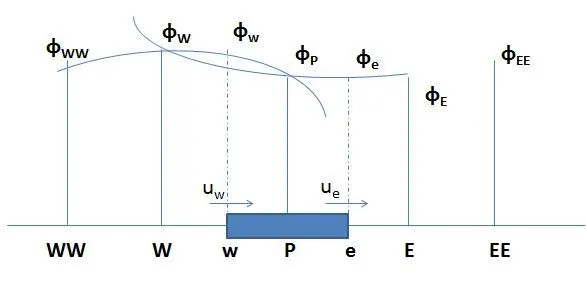
for `u _w >0 : phi_w rarr`is evaluated based on the values at WW,W and P
for `u_e > 0: phi_e rarr` is evaluated based on the Values at W, P and E
for`u_w<0;phi _w rarr` is evaluated based on the values at W, P and E
for `u_e < 0 : phi _e rarr` is evaluated based on the values at P,E and EE
`f_e rarr f_E + g_1(f_D-f_U) +g_2(f_(UU-fU))`
where,
`g_1 = ((x_e -x_U)(x_e - x_(UU)))/((x_(UU) -x_U ) (x_(UU) -x_D))`
`g_1 = ((x_e -x_U)(x_e - x_(D)))/((x_(UU) -x_U ) (x_(UU) -x_D))`
ADVANTAGES.
- It has an order of Accurarcy Three.
DISADVANTAGES.
- The Use of Quadratic Upstream Interpolation Convective Kinematics can lead to Subtle problems caused by Unbounded results.
- FLUX LIMITER.
For Convective Fluid Flow, It is Observed that the Lower Order Schemes are Usually Stable but Quite Dissipative in Nature around the points of Discontinuity or Shocks While the Higher Order Schemes are Unstable in nature and show Oscillations in the Vicinity of Discontinuities or Shocks. Highly Accurate and Oscillation-free Schemes are Known as High Resolution Schemes.
They Operate Functionally as a Switch and tune the numerical Fluxes Obtained from lower Order Schemes and Higher Order Schemes such that a lower Order scheme is empolyed near the discontinuity and High Order Scheme away from it.
In Order to make the Scheme TVD, must constrain or limit the range of possible values of the additional Convective Flux.
`f_e rarr f_P +1/2 phi (r) (f_E-f_P)`
Which was Orginally Introduced to make the Scheme Higher Order. Hence the function`psi (r)` is called as flux limiter function. Flux Limiter Functions are Used to fine tune the Higher Order and Lower Order Schemes in such a way that the resulting Scheme gives a higher order accurarcy in the smooth region of the flow and maintians first order accurarcy in the vicinity of shocks and discontinuities.
Consider 1D semi discrete Scheme.
`(du_i)/(dt) + 1/(Delta x_i)[ F(u_(i+1/2)) - F(u_(i-1/2))] = 0`
`F(u_(i+1/2)); F(u_(i-1/2))`
`F(u_(i+1/2) )rarr f_(i+1/2)^(low) - phi(r_i) (f_(i+1/2)^(low) -f_(i+1/2)^(high))`
`F(u_(i-1/2) )rarr f_(i-1/2)^(low) - phi(r_i) (f_(i-1/2)^(low) -f_(i-1/2)^(high))`
`f^(high) rarr`Low Precision, High Resolution Flux
`f^(low) rarr`High Precision, Low Resolution flux
`phi (r) rarr`Flux Limiter Function`
`r_i rarr (u_i - u_(i-1))/(u_(i+1) -u_i`
r represent the ratio of Successive Gradients on the Solution Mesh.
`phi(r)ge 0`
This is the Limiter Function Case.
If the Limiter Function = 0, there will be a low resolution and Sharp gradient.
If the Limiter Function >0 there will be a high resolution and positive gradient.