Project 2 - Rankine cycle Simulator

AIM  : 

• To create a Rankine Cycle Simulator using a MATLAB .

OBJECTIVES : 

• To calculate the each state points of Rankine Cycle  based on user inputs .
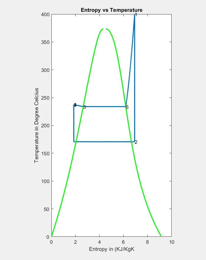
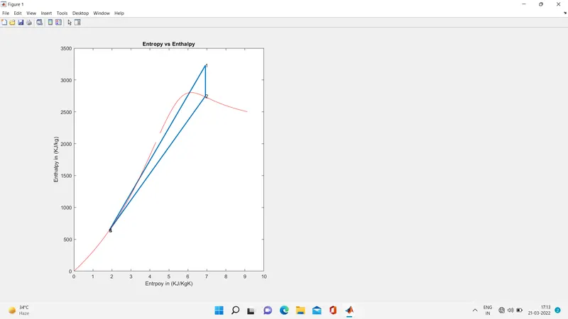
• To plot the corresponding T-s and h-s plots  for the given set of inputs .
• To calculate the Efficiency .

THEORY : 

1. RANKINE CYCLE :-  

• Rankine Cycle theory is introduced by William John Macquorn Rankine  in the year of 1859 .
• The Rankine Cycle is an idealized thermodynamic cycle describing the process by which certain heat engines , such as steam turbines or reciprocating steam engines , allow mechanical  work  to be extracted from a fluid as it moves between the heat source and heat sink .
• It is used  as a thermodynamic standard for rating the steam power  plants .

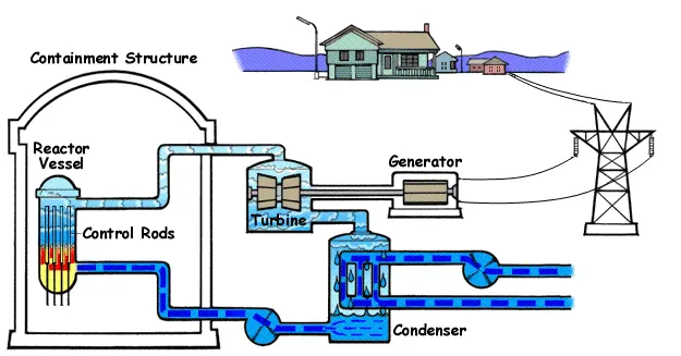
    2. LAYOUT OF RANKINE CYCLE  :

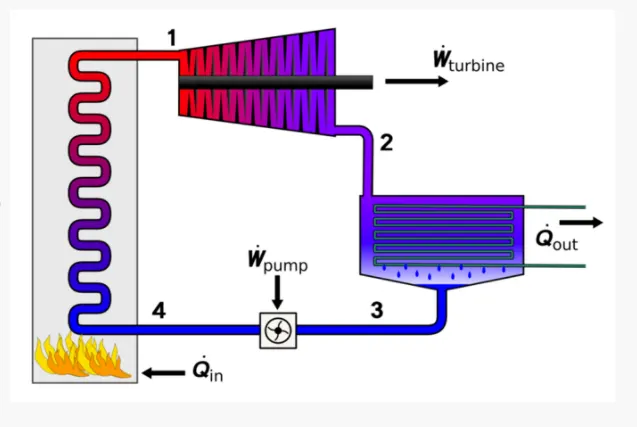
•  1. PUMP
•  2. BOILER 
•  3.TURBINE
•  4.CONDENSER .

• Heat  energy is supplied to a system via a boiler ,where the working fluid is converted to a high pressure gaseous state in order to turn a turbine .  
• After passing over the turbine the fluid is allowed to condense back into a liquid  state as waste heat energy is rejected before being returned to boiler , completing the cycle .
• Friction losses throughout the system are often neglected for the purpose of simplifying calculations as such losses are usually much less significant than thermodynamic losses , especially in larger system .

    3. WORKING PRINCIPLE : 

• There are four process in the Rankine cycle . They are , 
• process 1-2 : Isentropic  Expansion in a turbine .
• process 2-3 : Constant Pressure Heat Rejection in a condenser .
• process 3-4 : Isentropic Compression in a pump .
• process 4-1 : Constant Pressure Heat Addition  in a boiler .

1. Process  1-2 : ISENTROPIC EXPANSION IN A TURBINE : The dry saturated vapour expands throgh a turbine , generating power .This decreases the temperature and pressure of the vapour and some condensation may occur . This process is called as isentropic expansion . 
2. Process  2-3 : CONSTANT PRESSURE HEAT REJECTION IN A CONDENSER : Then the vapour exits from the turbine and enters the condenser ,so it is been condensated a while , at low pressure to become a saturated liquid . This prcoess is called as heat rejection .
3. Prcoess  3-4 : ISENTROPIC COMPRESSION IN A TURBINE  : The pressure of the condensate is raised in a feed pump, because of low specific volume of liquid the feed pump work is relatively small so the pump requires an input energy .
4. Process  4-1 : CONSTANT PRESSURE HEAT ADDITION IN A BOILER  : The high pressure liquid enters the bolier from the feed pump and is heated to the saturated temperature .Further addition of energy causes a evaporation of liquid until it is converted into a saturated steam .

EQUATIONS OF RANKINE CYCLE : 

(qin-qout)+(Win-Wout) = he-hi

Wpump = h2-h1

where h1 = hf 

         v1 = vf      for pressure respectively .

•  Heat addition in the boiler 

qin = h3 -h2 

• The work done from the turbine is given as 

Wout = h3 -h4 

• Heat rejection 

qout = h4 -h1

• The thermal efficiency 

Wnet = qin -qout = Wturb-Wpump

    4. A ANIMATED LAYOUT OF RANKINE CYCLE SIMULATOR :

ADVANTAGES : 

• The Thermal efiiciency is improved because average temperature of heat addition to cycle is increased .
• The Heating rate is reduced .
• The LP turbine blade height can be reduced because steam flow at lower stage is reduced .

MAIN PROGRAM : 

% A program to calculate the Rankine cycle simulator 

clear all
close all 
clc

% Rankine cycle simulator 
fprintf('1-2 Isentropic expansion in a turbine\n')
fprintf('2-3 Constant pressure heat rejection in a condenser\n')
fprintf('3-4 Isentropic compression in a pump\n')
fprintf('4-1 Constant pressure heat addition in a boiler\n')

% Inputs data to calculate the state points 

% Pressure in the turbine inlet 
p1 = 30;

% Temperature in the turbine inlet in degree  celcius 
T1 = 400;

% Pressure in the condenser Inlet 
p2 = 5;

% To calculate the state point 1 the datas are taken from XSteam files

% Calculate  the  Enthaply at pressure and Temperature
h1 = XSteam('h_pT',p1,T1);

% Calculate the Entropy at pressure and Temperature 
s1 = XSteam('s_pT',p1,T1);

% To calculate the State point 2  the datas are taken from XSteam files
s2  = s1;

% Calculate the saturated liquid Entropy at pressure 
sf2 = XSteam('sL_p',p2);

% Calculate the saturated vapour Entropy at pressure 
sg2 = XSteam('sV_p',p2);

% To calculate the Vapour fraction 
x2  = (s2-sf2)/(sg2-sf2);

% Calculate the saturated liquid Enthalpy at pressure 
hf2 = XSteam('hL_p',p2);

% Calculate the saturated vapour Enthalpy at pressure 
hg2 = XSteam('hV_p',p2);

% Therefore
h2 = hf2 + (x2*(hg2-hf2));
h2 = hg2;

% Calculate the temperatrure 
T2 = XSteam('T_hs',h2,s2);

% To calculate the state point 3 the datas are taken from XSteam files
p3 = p2;
T3 = T2;
% Calculate the saturated liquid Entropy at pressure 
s3 = XSteam('sL_p',p3);

% Calculate the saturated liquid Enthaply at pressure
h3 = XSteam('hL_p',p3);

% To calculate the state point 4 the datas are taken from XSteam files
p4  = p1;
s4  = s3;

% To calculate the Temperature for the state points 1 2 3 and 4
Cp4 = XSteam('Cp_ps',p4,s4);
Cv4 = XSteam('Cv_ps',p4,s4);
gamma = Cp4/Cv4;
r   = (gamma-1)/gamma;
T4  = T3*(p4/p3)^r;

% To calculate the output values

% Calculate the work done in the turbine 
Wt = h1 - h2;

% Calculate the work done in the pump 

% calculate the saturated vapour liqiud at pressure 
v3 = XSteam('vL_p',p3);
Wp = v3*(p1-p2)*100;
h4 = Wp + h3;

% Calculate the net work unit
W_net = Wt-Wp;

% Calculate the heat supplied 
Qs = h1 - h4;

% Calculate the Thermal efficiency 
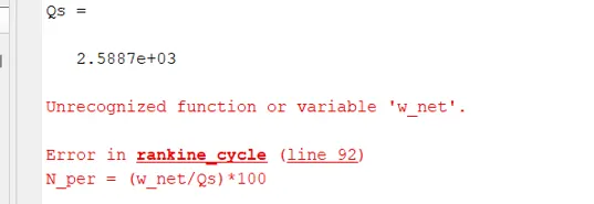
N_per = (W_net/Qs)*100;

% calculate the steam rate value for per second
steam_rate = 3600/(Wt-Wp);

% To calculate the state point 5 and 6 the datas are taken from XSteam files
T5 = XSteam('Tsat_p',p1);
T6 = T5;

% Calculate the saturated liquid Entropy at pressure 
s5 = XSteam('sL_p',p1);

% Calculate the saturated vapour Entropy at pressure 
s6 = XSteam('sV_p',p1);

% Calculate the saturated liquid Enthaply at pressure
h5 = XSteam('hL_p',p1);

% Calculate the saturated vapour Enthalpy at pressure
h6 = XSteam('hV_p',p1);

% Plotting the T-S Diagram 
subplot(1,3,1)
T_rankine = linspace (T5,T1,3000);
for i = 1:length(T_rankine)
    s_rankine(i) = XSteam('s_pT',p1,T_rankine(i));
end
plot([s1 s2 s3 s4 s5 s6 s_rankine],[T1 T2 T3 T4 T5 T6 T_rankine],'linewidth',2);
hold on 
T_curve = linspace(1,400,350);
for i = 1:length(T_curve)
    s_l(i) = XSteam('sL_T',T_curve(i));
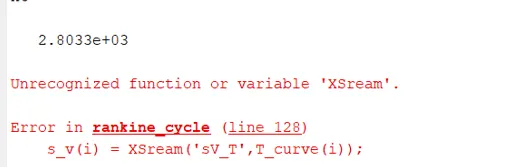
    s_v(i) = XSteam('sV_T',T_curve(i));
    h_l(i) = XSteam('hL_T',T_curve(i));
    h_v(i) = XSteam('hV_T',T_curve(i));
end
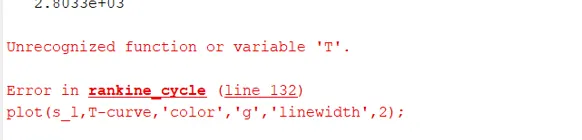
plot(s_l,T_curve,'color','g','linewidth',2);
plot(s_v,T_curve,'color','g','linewidth',2);
text(s1,T1,'1')
text(s2,T2,'2')
text(s3,T4,'3')
text(s4,T4,'4')
text(s5,T5,'5')
text(s6,T6,'6')
title('Entropy vs Temperature');
xlabel('Entropy in (KJ/KgK');
ylabel('Temperature in Degree Celcius');

% plotting the H-S diagram 
subplot (1,2,1)
plot([s1 s2 s3 s4 s1],[h1 h2 h3 h4 h1],'linewidth',2)
hold on 
plot(s_v,h_v,'color','r')
plot(s_l,h_l,'color','r')
text(s1,h1,'1')
text(s2,h2,'2')
text(s3,h3,'3')
text(s4,h4,'4')
title('Entropy vs Enthalpy')
xlabel('Entrpoy in (KJ/KgK)')
ylabel('Enthalpy in (KJ/Kg)')

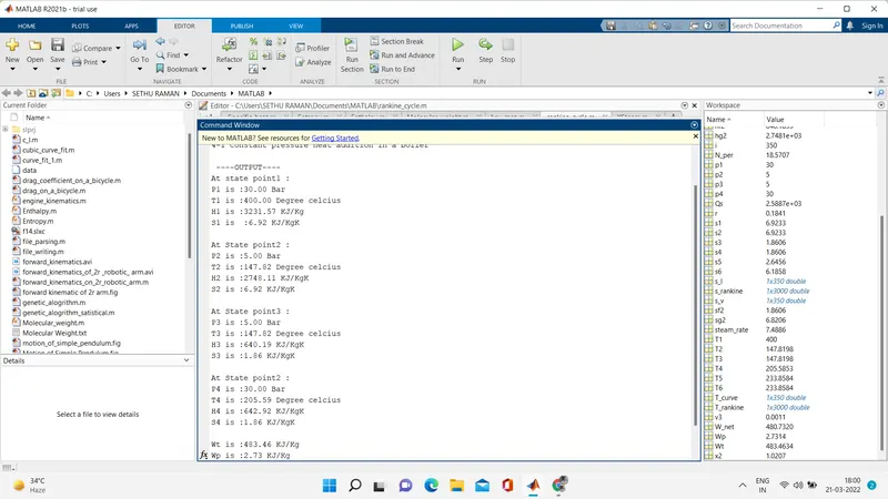
% Print all the State value in the command window 
fprintf('\n ----OUTPUT----\n')
fprintf('At state point1 :\nP1 is :%4.2f Bar\nT1 is :%4.2f Degree celcius\nH1 is :%4.2f KJ/Kg\nS1 is  :%4.2f KJ/KgK\n\n',p1,T1,h1,s1)
fprintf('At State point2 :\nP2 is :%4.2f Bar\nT2 is :%4.2f Degree celcius\nH2 is :%4.2f KJ/KgK\nS2 is :%4.2f KJ/KgK\n\n',p2,T2,h2,s2)
fprintf('At State point3 :\nP3 is :%4.2f Bar\nT3 is :%4.2f Degree celcius\nH3 is :%4.2f KJ/KgK\nS3 is :%4.2f KJ/KgK\n\n',p3,T3,h3,s3)
fprintf('At State point2 :\nP4 is :%4.2f Bar\nT4 is :%4.2f Degree celcius\nH4 is :%4.2f KJ/KgK\nS4 is :%4.2f KJ/KgK\n\n',p4,T4,h4,s4)
fprintf('Wt is :%4.2f KJ/Kg\nWp is :%4.2f KJ/Kg\nWnet is :%4.2f KJ/Kg\nNtherm is :%4.2f percent\nS.S.C is :%4.2f Kg/KWh',Wt,Wp,W_net,N_per,steam_rate)

OUTPUTS : 

    

CODE EXPLANATION : 

• The program starts with 'Clear all ' 'close all ' and 'clc' .
• 'Clear all ' command is used to clear  all the  varaibles from the workspace .
• 'Close all ' command is used to close the plots and figures .
• 'Clc command is used to clear  the command window .
• Then the Input Varaibles of p1 T1 and p2 which is  pressure and temperature of  inlet turbine and inlet condenser are given .
• The values of Enthalpy, Entropy is been calculated in the state point1 .
• With the help of XSteam file datas , the datas of h_pt, sV_p,hl_p,sL_p, is taken 
• Respectively remaining state points of 2, 3, 4 ,5 ,6 of input values is  taken from the XSteam files .
• Then with respect all the entropy, enthalpy, pressure ,and temperature is been calculated.
• Then in the stage of state 2  at condsener inlet the high pressure steam is converted to the low pressure water .Therefore the values of entropy , enthalpy for the saturated vapour and water is been calculated .
• At stage of state 3  the water is condensed back to its staturation temperature through the pump  and state 4 Cp/Cv = gamma is considered to calculate the temperature of T4.
• Then Thermal efficiency , work done of the rankine cycle is calculation with the required equations.
• And finally plotting is done for both T-S and H-S curves .
• Output of the Rankine Cycle simulation is been displayed in the command window .                                                                                                                                                                                     

ERRORS :