Week 4.1 - Genetic Algorithm

AIM :

• To optimise the Stalagmite function and to find the Global maxima of the function .

OBJECTIVES :

• To write the code in matlab to optimise the stalagmite function and to find the global maxima of the function .
• To explain the concept of genetic alogrithm and syntax for the ga in matlab .
• To plot the graphs and find the F maximum and no of iteration .

THEORY : GENETIC ALOGRITHM

• Inspired by charles Darwin 's theory.
• A genetic alogrithm is a metaheuristic inspired by the process of natural selection that belongs to the lager class of evolutionary alogrithm .
• Genetic alogrithm are most commonly used to generate high quality solution to optimization on biologically inspired operators such as mutation , crossover , and selection .

HOW EVOLUTION WORKS :

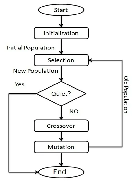
• 1. SELECTION :
• The of idea of selection process is to select the fittest individuals and let them pass their geners to the next generation .
• Tow pairs of generation (parents ) are selected based on the their fitness scores.
• Individuals with high fitness have more chances to be selected for the reproduction.

• 2.CROSSOVER :
• Crossover is the significant phase in the genetic alogrithm .
• For each to be mated, a crossover points is chosen at random form within the genres .

• 3.MUTATION :
• Mutation occurs to maintain the diversity withinn the population and prevent premature convergence.

FLOWCAHRT OF THE GENETIC ALOGRITHM :

SYNTAX FOR GENETIC ALOGRITHM :

• fun = objective function ,
• nvars = numbers of varaibles,
• A,b = linear inequality constraints ,
• Aeg,beq = linear equality constraints ,
• lb = lower bounds,
• ub = upper bounds ,
• nonlcon = nonlinear constraints,
• intcon = indices of integer varaubles ,
• options = optimization options,
• x = solutions,
• fval = objective function value at solution ,
• exitflag = reason ga stopped ,
• output = information abut the optimization process
• population = find population
• sxores = find scores .

STALAGMITE THEORY :

• A stalagmite function is an upward - growing mound of minerals desposits that have precipitated from the water dripping onto the floor of a cave .
• Most stalagmite function have rounded or flattered tips .

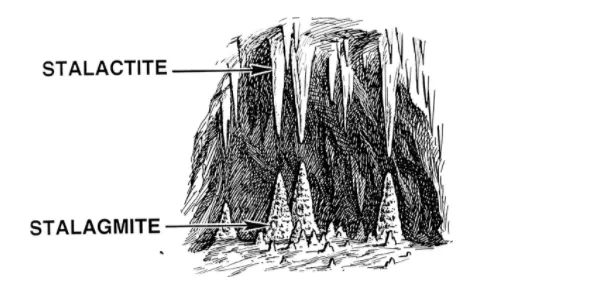
• A stalagmite function generally refers to the function with which we are generating values over a stalagmite kind of surface for finding out the local and global maxima and minima of that particular given function .

function [v] = stalagmite(input_vector)
 x = input_vector(1);
 y = input_vector(2);
 f1 = (sin(5.1*pi*x+0.5)).^6;
 f2 = exp((-4*log(2)*(x-0.0667).^2))/0.64;
 f3 = (sin(5.1*pi*y+0.5)).^6;
 f4 = exp((-4*log(2)*(y-0.0667).^2))/0.64;

 v = -(f1*f2*f3*f4);
end​

• we are using negative sign (-Ve) in this function ,so that the plot will be reversed as we can find the global maxima of the given function using ga .

PROGRAM :

% A program to optimise the stalagmite function and find global maxima 
clear all 
close all 
clc

% Defining our search space 
x = linspace(0,0.6,150);
y = linspace(0,0.6,150);
num_case = 50;

% Creating the 2Dimensional array 
[xx,yy] = meshgrid(x,y);

% Evaluating the stalagmite function 
for i = 1:length(xx);
    for j = 1:length(yy);
        input_vector(1) = xx(i,j);
        input_vector(2) = yy(i,j);
        f(i,j) = stalagmite(input_vector);

    end 
end 
 % study 1 - unbounded behaviour 
 tic 
 for i = 1:num_case
     [result,fopt(i)] = ga(@stalagmite,2);
     xopt(i) = result(1);
     yopt(i) = result(2);
 end
%  study_time 1 = toc 

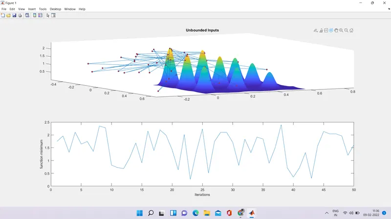
 figure(1)
  subplot(2,1,1)
  hold on 
  surfc(x,y,-f)
  shading interp
  plot3(xopt,yopt,-fopt,'marker','o','markersize',4,'markerfacecolor','r')
  title('Unbounded Inputs')
  subplot(2,1,2)
  plot(-fopt)
  xlabel('Iterations')
  ylabel('function minimum')

% study 2 - unbounded behaviour with upper an lower bound 
 tic 
 for i = 1:num_case
     [result,fopt(i)] = ga(@stalagmite,2,[],[],[],[],[0;0],[0.6;0.6]);
     xopt(i) = result(1);
     yopt(i) = result(2);
 end 
 % study_time 2 = toc

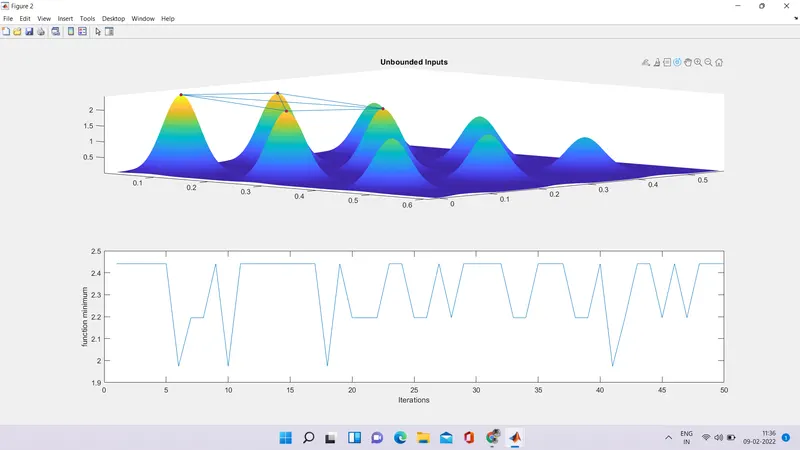
figure(2)
  subplot(2,1,1)
  hold on 
  surfc(x,y,-f)
  shading interp
  plot3(xopt,yopt,-fopt,'marker','o','markersize',4,'markerfacecolor','r')
  title('Unbounded Inputs')
  subplot(2,1,2)
  plot(-fopt)
  xlabel('Iterations')
  ylabel('function minimum')

% study 3 - increased inital population 
tic 
options = optimoptions('ga')
options = optimoptions(options,'populationsize',200)

for i = 1:num_case
    [result,fopt(i)] = ga(@stalagmite,2,[],[],[],[],[0;0],[0.6;0.6],[],[],options);
    xopt(i) = result(1);
    yopt(i) = result(2);
end 

% study _time 3 = toc 

  figure(3)
  subplot(2,1,1)
  hold on 
  surfc(x,y,-f)
  shading interp
  plot3(xopt,yopt,-fopt,'marker','o','markersize',4,'markerfacecolor','r')
  title('Unbounded Inputs')
  subplot(2,1,2)
  plot(-fopt)
  xlabel('Iterations')
  ylabel('function minimum')

CODE EXPLANATION :

• The code starts with 'clear all', 'close all','clc' commands respectively .
• 'clear all' command is used to clear the workspace data .
• 'close all'command is used to close the plots and figure data .
• 'clc' command is used to clear the datas in the command window .
• 'linspace 'command is used to create the spaced sequence in a specified intervals. so in this the given inputs of x ,y values are considered inbetween interval is 150.
• 'meshgrid ' command is used to evaluate the functions of two varaibles and three -dimensional mesh /surface plots.
• The tic - toc is used to measure the time for running the program.
• The label and title are used to understand in a easier way , so that it looks neat and clean .
• Finally all 3 studies of global maxima have been runned sucessfully .

RESULT :

STUDY 1 :

STUDY 2 :

STUDY 3 :

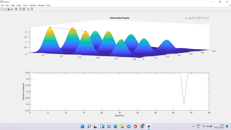
• It is noted , that whenever we re - run the program the study 1 and study 2 varies a lot but , study 3 shows the clear result of global maxima .

ERROR :

• Error faced while working on the program . xpot instead of xopt.