Week 9 - FVM Literature Review

AIM

• To explain the working of the Finite Volume Method (FVM) and its major differences as compared to the Finite Difference Method (FDM).
• To explain the role of different Gradient Schemes and Interpolation Schemes along with the significance of Flux limiters.

THEORY

In computational fluid dynamics, there are 3 numerical method-based solvers to solve the governing Navier-Stokes equations these are:

1. Finite Element Method

2. Finite Difference Method

3. Finite Volume Method

1. Finite Element Method

FEM subdivides a large system into smaller, simpler parts that are called finite elements. This is achieved by a particular space discretization in the space dimensions, which is implemented by the construction of the mesh of the object: the numerical domain for the solution, which has a finite number of points.

2. Finite Difference Method

In FDM, both the spatial domain and time interval (if applicable) are discretized, or broken into a finite number of steps, and the value of the solution at these discrete points is approximated by solving algebraic equations containing finite differences and values from nearby points. The properties are assumed to be concentrated at the nodes.

3. Finite Volume Method

In the finite volume method, volume integrals in a partial differential equation that contain a divergence term are converted to surface integrals, using the divergence theorem. Finite volume refers to the small volume surrounding each node point on a mesh. Properties are assumed to be concentrated at the geometric center of the volume concerned.

Drawbacks of FDM

1. FDM can be used only if the grids are aligned in a coordinate system. In case of unstructured meshes, error correction is needed for uniform calculation of the field variables.
2. This correction is done by a method known as Variable Transformation. This creates an alternative coordinate system in terms `eta` and `epsilon` that is a function of the generic coordinate system. However, as we solve more complex geometries, this transformation becomes very tedious and convoluted.

To address this problem Finite Volume Method is considered.

Finite Volume Method

The finite volume method (FVM) is a discretization technique for partial differential equations arising from physical conservation laws. In fluid dynamics, the entire fluid domain is divided into a finite number of cells. FVM uses a volume integral formulation of the problem with a finite partitioning set of volumes to discretize the equations.

In the finite volume method, volume integrals in a partial differential equation that contain a divergence term are converted to surface integrals, using the divergence theorem. Finite volume refers to the small volume surrounding each node point on a mesh. The field variables are assumed to be concentrated at the geometric center of the volume concerned. These variables are then evaluated as fluxes at the surfaces of each finite volume. Because the flux entering a given volume is identical to that leaving the adjacent volume, these methods are conservative.

FVM rests on the mathematical foundation of the Gauss Divergence Theorem.

Gauss Divergence theorem

The theorem states that the surface integral of a vector field over a closed surface, which is called the flux through the surface, is equal to the volume integral of the divergence over the region inside the surface.

`oint_V (grad . F) dV = oint_S (F. hat n) dS`

The theorem allows the construction of dynamic equations for volume-averaged variables.

Working of FVM

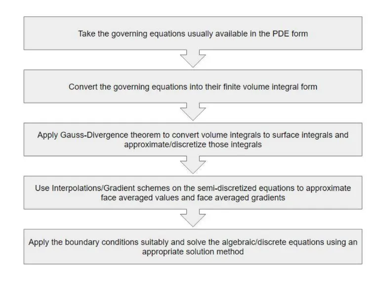
Hence, we arrive at the conclusion that the Finite Volume Method is a much more reliable and accurate method for complex 2D/3D geometries as compared to the Finite Difference Method. Below are the major differences between FVM and FDM

Finite Difference Method	Finite Volume Method
Governing Equations are in differential form	Governing equations are in integral form
The field variables are computed at each node.	The field variables are computed at the cell centroids.
A structured grid in the generic cartesian coordinate system is required. For complex geometries, Variable Transformation needs to be adapted for error correction which is not feasible.	Can solve for unstructured grids due to the assumption of volume around each node, making it an optimum choice to solve complex geometries.
All field variables need to be differentiable and continuous over the entire domain making it unsuitable for solving for discontinuous functions.	The method can handle the discontinuity due to the integral form of the governing equations.
The method does not ensure conservation.	The method ensures conservation in the local as well as global domain.

Below is the 1D Heat equation example to further explain the FV method.

1. Once we have this integral form of the equation.
2. Apply Gauss divergence theorem
3. We get a discretized form of algebraic equations that can be solved.

Consider a steady-state heat conduction equation with heat generation:

`del/(del x) (alpha. (delT)/(delx)) + S =0`

S is the source term

`alpha` is thermal diffusivity term

`(delT)/(delx)` is the temperature gradient along the x direction

Taking the conservation equation validated at single point and if it is validated at single point then it is validated at entire volume and in this entire volume properties are conserved.

Multiplying the equation by `dV, we get

`int(del/(del x) (alpha. (delT)/(delx)) + S) dV =0`

`int(del/(del x) (alpha. (delT)/(delx))) A.dx+ intS dV =0`

`[(alpha. (delT)/(delx))]_w ^e + barS dV =0`

`alphaA [(T_E-T_P)/(trianglex)] - alphaA [(T_P-T_W)/(trianglex)] + barSdV = 0`

The source term is to be added in a cell, if it is a function of temperature we have to linearize it. If `alpha` is a function of temperature we have to linearize this also.

`bar S Rightarrow S_u + S_pT_p`

Gradient Schemes

To solve for the gradient terms (like Pressure) Gradient Schemes are used to address the discontinuity that would be caused if the same pressure term is considered with the new velocity terms in the governing equations. The gradient are evaluated at cell centroids.

1. Gauss gradient scheme

This scheme approximates the gradient/slope using the Gauss Divergence Theorem. The gradients are computed from face values that require Interpolation.

2. Least Squared gradient scheme

The scheme approximates the gradient at the cell centroids using neighbor cell centroid values and not face values.

Interpolation Schemes

Interpolation schemes are used to evaluate the face values that arise as a part of the convective flux and diffusive flux terms in the discretization of NS equations in the integral form. The schemes find values of volume integrals required at points other than nodes.

Some Interpolation Schemes used in FVM are -

1. Upwind interpolation scheme

2. Linear interpolation scheme

3. Linear Upwind Differencing

4. Quadratic Upwind Interpolation for Convective Kinematics (QUICK) scheme

5. Total Variation Diminishing (TVD) scheme

Flux Limiters

Flux limiters are used for the second and higher-order interpolations, that predict face values based on gradients at centroids of a cell.

Due to the presence of sharp gradients present in the flow, the flux terms tend to overshoot and exceed the local minima/maxima and create a new minima/maxima causing disruption in the global domain and spurious oscillations in the solution.

To avoid this flux limiter functions are introduced in the equation such that it monitors the ratio of successive gradients. The functions operate functionally as a switch and tune the numerical fluxes obtained from the lower order scheme and higher order scheme such that near the discontinuity lower order (stable) scheme is employed and away from it higher order (accurate) scheme is employed.

Note that flux limiters are also referred to as slope limiters because they both have the same mathematical form, and both have the effect of limiting the solution gradient near shocks or discontinuities. In general, the term flux limiter is used when the limiter acts on system fluxes and slope limiter is used when the limiter acts on system states (like pressure, velocity etc.).

THE END