Week 5.1 - Mid term project - Solving the steady and unsteady 2D heat conduction problem
AIM
To solve the 2D heat conduction equation for the steady and unsteady state using various iterative solvers such as Jacobi, Gauss-Seidel, and Successive over relaxation methods using MATLAB.
THEORY
The 2-D Heat Conduction equation (Fourier's Law) defines the heat transfer through a 2-dimensional surface. The partial differential equation defines the propagation of heat through the surface over time. The propagation of heat is represented in two standard equations.
i. Steady State Equation - The steady state equation defines the diffusion of heat through the surface which is independent of time. That is, it explains the flow that must have taken place after equilibrium is attained. Hence making the temperature function.
`(del^2T)/(delx^2) + (del^2T)/(dely^2) = 0`
ii. Unsteady State Equation - The unsteady state equation precisely defines the heat conduction through the surface, evolving with time. This explains the propagation of heat from t=0 as the conduction begins. Hence, making it time-dependent.
`(del^2T)/(delx^2) + (del^2T)/(dely^2) = 1/alpha ((delT)/(delt))`
where `alpha` is the thermal diffusivity.
The solutions methodology adopted to solve the above PDE is executed in the following steps
1. Discretization
The above PDE is discretized using the Central Differencing Scheme. Upon discretization of the individual terms, we get
`((del^2T)/(del^2x))_(i,j)^n = (T_(i-1,j)^n - 2T_(i,j)^n +T_(i+1,j)^n)/(trianglex)^2`
`((del^2T)/(del^2y))_(i,j)^n = (T_(i,j-1)^n - 2T_(i,j)^n +T_(i,j+1)^n)/(triangley)^2`
`(delT)/(delt) = (T_(i,j)^(n+1) - T_(i,j)^(n))/(trianglet)`
Here, `T_(i,j)^n = T_p` = Temperature at P at time n
`T_(i-1,j)^n = T_L`= Temperature at left node L at time n
`T_(i+1,j)^n = T_R`= Temperature at right node R at time n
`T_(i,j-1)^n = T_T`= Temperature at top node T at time n
`T_(i,j+1)^n = T_B`= Temperature at bottom node B at time n
a. For Steady State we have
`(T_(i-1,j)^n - 2T_(i,j)^n +T_(i+1,j)^n)/(trianglex)^2 +(T_(i,j-1)^n - 2T_(i,j)^n +T_(i,j+1)^n)/(triangley)^2 =0`
b. For Unsteady State we have
`(T_(i-1,j)^n - 2T_(i,j)^n +T_(i+1,j)^n)/(trianglex)^2 +(T_(i,j-1)^n - 2T_(i,j)^n +T_(i,j+1)^n)/(triangley)^2 = 1/alpha((T_(i,j)^(n+1) - T_(i,j)^(n))/(trianglet))`
2. Iterative Solvers
Upon discretization, we get the linear equation. The equations above can be solved using explicit and implicit techniques. However, the Steady State Equation is solved using the implicit technique and the Unsteady State Equation is solved using both the explict and implicit techniques.
Based on the Implicit Techniques we have three solvers as follows
a. Jacobi Iterative Solver
In this method, the temperature at n+1th iteration is found using old values of the temperature defined at nth iterations. Using the approximation obtained iterations procedure it continued until the desired accuracy of the solution is obtained.
b. Gauss-Seidel Iterative Solver
In this type of iterative solver, the temperature at n+1 iterations uses values of n+1 iterations that have already been computed. Through this method, old approximated values are overwritten with new approximate values for the iterations performed. Unlike Jacobi, Gauss-Seidel requires one storage vector which can be overwritten with each computation. This helps the solution to converge faster than the Jacobi method.
c. Successive over-relaxation Iterative Solver
In this type of iterative solver relaxation factor is used which helps in increasing the convergence rate. It goes by the formula -
`T_(i,j)^(n+1) = (1-omega)*T_(i,j)^n + omega*T (text(gauss-seidel))`
where `omega` is the relaxation factor. Its range is from 0-2
when `omega` is between 0-1 it is called under relaxed state.
This condition is used when the temperature gradient is high and due to this condition, the time step does not overshoot and helps to converge at a faster rate.
when `omega` is between 1-2 it is called over-relaxed state.
This condition is used when the temperature gradient is low and due to this condition, larger time steps are used to obtain the steady state i.e., for the values to converge at a faster rate.
For Steady State Equation, we have the following
Jacobi Method
`T_P^(n+1) = 1/k((T_L^n+T_R^n)/(trianglex)^2 + (T_T^n+T_B^n)/(triangley)^2)`
Gauss-Seidel Method
`T_P^(n+1) = 1/k((T_L^(n+1)+T_R^n)/(trianglex)^2 + (T_T^(n+1)+T_B^n)/(triangley)^2)`
SOR Method
`T_P^(n+1) = (1-omega)*T_P^n + omega*T(GS)`
Note - Here `k = 2(((trianglex)^2 + (triangley)^2)/((trianglex)^2(triangley)^2))`
For Unsteady State Equation, we have the following
Jacobi Method
`T_P^(n+1) = 1/(1+2k1+2k2)(T_P^n +k1(T_L^n+T_R^n) + k2(T_T^n+T_B^n))`
Gauss-Seidel Method
`T_P^(n+1) = 1/(1+2k1+2k2)(T_P^n +k1(T_L^(n+1)+T_R^n) + k2(T_T^(n+1)+T_B^n))`
SOR Method
`T_P^(n+1) = (1-omega)*T_P^n + omega*T(GS)`
Note - Here `k = alpha(trianglet)/(trianglex^2)`
MATLAB PROGRAM
1. Assumptions and Input Parameters
Top Boundary = 600 K
Bottom Boundary = 900 K
Left Boundary = 400 K
Right Boundary = 800 K
L=1m
Absolute Error = 1e-4
2. MATLAB Code
a. Steady State
i. Main Code
%Code to study the behaviour of steady state analysis
%using implicit method.
clear all
close all
clc

%Defining spacial domain
nx = 10;ny=10;
L=1;
x = linspace(0,L,nx);
y = linspace(0,L,ny);

%grid size
dx = x(2)-x(1);
dy = y(2)-y(1);

% defining temperature
t = 300* ones(nx,ny);
% [t] = 300*meshgrid(x,y);
t(end,:) = 900;        % top face
t(1,:) = 600;          % bottom face
t(:,1) = 400;          % left face
t(:,end) = 800;        % right face

% Corner temperatures
t(1,1)= (t(1,2)+t(2,1))/2;
t(end,1) = (t(end,2)+t((end-1),1))/2;
t(1,end)= (t (1,(end-1))+t(2,end))/2;
t(end,end)=(t((end-1),(end))+ t(end,(end-1)))/2;

%Tolerance
tol=1e-4;

k = 2*(dx^2+dy^2)/(dx^2*dy^2);
told=t;

%Function to calculate the temperature of Steady state using iterative solvers
[error_j,iter1] = fun_steady_state_jacobi(nx,ny,t,told,k,dx,dy,tol);
[error_gs,iter2] = fun_steady_state_gs(nx,ny,t,told,k,dx,dy,tol);
[error_sor,iter3] = fun_steady_state_sor(nx,ny,t,told,k,dx,dy,tol);
ii. Function Codes
Jacobi Iterative Solver
%Function for calculation of Steady State using Jacobi Method
function [error_j,iter1] = fun_steady_state_jacobi(nx,ny,t,told,k,dx,dy,tol)


        %defining iteration variable
        iter1 = 0;
        % Assumed error value
        error_j = 9e9;

    %convergence loop
    while (error_j>tol)

                %Iteration loop
                for i = 2:(nx-1)
                     for j = 2:(ny-1)

                        %Formula for calculation of temperature at each
                        %grid point

                         H = (told(i-1,j) + told(i+1,j))/dx^2;
                         V = (told(i,j-1) + told(i,j+1))/dy^2;

                        t(i,j) = (H +V)/k;

                    end
                end

                %error for each iteration
                error_j = max(max(abs(told-t)));

                %updating the temperature values for the next iteration.
                told = t;

                %incrementing iter variable
                iter1 = iter1+1;
    end

    % Filled Contour Plot
    figure(1)
    [C,h]=contourf(t);
    clabel(C,h);
    colormap(jet);
    axis ij;
    title_text = sprintf('Number of Iteration = %d',iter1);
    title(title_text);

end
Gauss-Seidel Solver
%Function for calculation of Steady State using GS Method
function [error_gs,iter2] = fun_steady_state_gs(nx,ny,t,told,k,dx,dy,tol)


        %defining iteration variable
        iter2 = 0;
        % Assumed error value
        error_gs = 9e9;

    %convergence loop
    while (error_gs>tol)

                %Iteration loop
                for i = 2:(nx-1)
                     for j = 2:(ny-1)

                        %Formula for calculation of temperature at each
                        %grid point

                         H = (t(i-1,j) + told(i+1,j))/dx^2;
                         V = (t(i,j-1) + told(i,j+1))/dy^2;

                        t(i,j) = (H +V)/k;

                    end
                end

                %error for each iteration
                error_gs = max(max(abs(told-t)));

                %updating the temperature values for the next iteration.
                told = t;

                %incrementing iter variable
                iter2 = iter2+1;
    end

    % Filled Contour Plot
    figure(2)
    [C,h]=contourf(t);
    clabel(C,h);
    colormap(jet);
    axis ij;
    title_text = sprintf('Number of Iteration = %d',iter2);
    title(title_text);

end
SOR Iterative Solver
%Function for calculation of Steady State using SOR Method
function [error_sor,iter3] = fun_steady_state_sor(nx,ny,t,told,k,dx,dy,tol)


        %defining iteration variable
        iter3 = 0;
        %Assumed error value
        error_sor = 9e9;
        %omega value
        omega = 1.15;

    %convergence loop
    while (error_sor>tol)

                %Iteration loop
                for i = 2:(nx-1)
                     for j = 2:(ny-1)

                        %Formula for calculation of temperature at each
                        %grid point

                         H = (t(i-1,j) + told(i+1,j))/dx^2;
                         V = (t(i,j-1) + told(i,j+1))/dy^2;

                        t_gs(i,j) = (H +V)/k;
                        t(i,j) = (1-omega)*(told(i,j))+omega*t_gs(i,j);

                    end
                end

                %error for each iteration
                error_sor = max(max(abs(told-t)));

                %updating the temperature values for the next iteration.
                told = t;

                %incrementing iter variable
                iter3 = iter3+1;
    end

    % Filled Contour Plot
    figure(3)
    [C,h]=contourf(t);
    clabel(C,h);
    colormap(jet);
    axis ij;
    title_text = sprintf('Number of Iteration = %d',iter3);
    title(title_text);

end
iii. Explanation
1. Firstly, the basic geometry is defined in the Main Code. This includes the grid size and total dimensions of the 2D surface.
2. After defining the geometry, the input parameters are defined. The input parameters are the boundary condition of the surface. This includes the temperature at the edges as given in the problem. and the temperatures at the corners are assumed as the average of the previous grid points.
3. Furthermore, convergence conditions are also defined (i.e. tolerance) along with k value as calculated by the derivations in the theory. After the function codes are called for their respective iterative solver.
4. In the function codes there is a similar structure followed apart from the difference in the formula of the iterative solvers itself as derived in the previous section.
5. The function code primarily follows 2 loops to calculate the 2D steady-state equation. After defining the initial error value and iteration variable, the while loop and for loop is used to achieve a solution. The initial iteration variable is taken as 0 and the error value is assumed as 9e9 as given in the problem.
6. The while loop is used to reach convergence (convergence loop), i.e. until the error value (T at n+1 iteration - T at n iteration) is less than the given error tolerance value the calculation will keep going.
7. The calculation is done with the for loop which is the iteration loop. The for loop calculates the temperature across all the grid points from the second to the second last. Note that the temperature at the first and last grids are already defined as boundary conditions across both x and y axes.
8. After every error calculation the old temperature has to be updated as the new temperature in order to achieve convergence. This update must be done after the calculation as it will give 0 error if it is calculated after the update of temperature.
9. As the new temperature gets calculated the iteration proceeds and hence the iteration value is updated to achieve the final number of iterations required to solve the problem.
10. Note that as the theory suggests, the Jacobi requires the highest number iterations, followed by the Gauss-Seidel and then SOR. It is discussed in the coming section.
b. Unsteady State
EXPLICIT METHOD
i. Main Code
%Code to study the behaviour of transient state analysis using explicit method.
close all
clc

%Defining spacial domain
nx = 10;ny=10;
L=1;
x = linspace(0,L,nx);
y = linspace(0,L,ny);

%grid size
dx = x(2)-x(1);
dy = y(2)-y(1);

% defining temperature
T = 300* ones(nx,ny);
% [t] = 300*meshgrid(x,y);
T(end,:) = 900;        % top face
T(1,:) = 600;          % bottom face
T(:,1) = 400;          % left face
T(:,end) = 800;        % right face

% Corner temperatures
T(1,1)= (T(1,2)+T(2,1))/2;
T(end,1) = (T(end,2)+T((end-1),1))/2;
T(1,end)= (T (1,(end-1))+T(2,end))/2;
T(end,end)=(T((end-1),(end))+ T(end,(end-1)))/2;

%Tolerance
tol=1e-4;
error = 9e9;

alpha = 1.1;
Told=T;
Tinitial =T
dt = 0.001;
nt=1400

%k value is the CFL number
k1= alpha*(dt/dx^2);
k2= alpha*(dt/dy^2);

   iter = 1;
   %Time loop
        for K=1:nt

                 %Iteration loop
                 for i = 2:(nx-1)
                     for j = 2:(ny-1)

                         %Formula for calculation of temperature at each grid point

                         H = Told(i-1,j) - 2*Told(i,j) + Told(i+1,j);
                         V = Told(i,j-1) - 2*Told(i,j) + Told(i,j+1);

                         T(i,j) = Tinitial(i,j) + (k1*H + k2*V);

                      end
                  end

                  %error for each iteration
                  error = max(max(abs(Told-T)));

                  %updating the temperature values for the next iteration.
                  Told = T;

                  %incrementing iter variable
                  iter = iter+1;

      Tinitial = T

            % Filled Contour Plot
            figure(1)
            contourf(x,y,T)
            clabel(contourf(x,y,T))
            colorbar
            colormap(jet)
            set(gca, 'ydir', 'reverse')

            xlabel('X-Axis')
            ylabel('Y-Axis')
            title(sprintf('No. of Unsteady Iterations (EXPLICIT) = %d', iter));


        end
ii. Explanation
1. In the Explicit Method, there are no separate main and function codes as only one solver is used. The explicit method in the unsteady equation does not need the iterative solver to solve the problem as all the required unknowns are already known. Hence, the calculation is done with the Time loop and the Iteration loop. There is no convergence loop as convergence is noticeably achieved at high time steps.
2. Similar to the Steady State equation the geometry is defined along with the grid size and the temperature matrix.
3. Then the boundary conditions are defined along with the dt value. As this is a time-dependent problem, the CFL numbers are defined both for the x and y axes terms as k1 and k2. Note that k1+k2 < 0.5 for the solution to achieve convergence.
4. The iteration loop solves the heat equation formula geometrically across all the nodes. The formula solves the temperature at each node at each time step based on the previous time step.
5. The time loop carries out the simulation up to 1400 time steps, which is assumed sufficient to achieve convergence. As the time loop needs to be solved Tinitial =T is assumed at 1st-time step. This repeats for each node for every time step.
6. The error is calculated the same way and then the temperature is updated for every node and then for every time step.
7. The contour map is plotted by realigning the y axis with help of the color map which provides a definitive gradient.
IMPLICIT METHOD
i. Main Code
%Code to study the behaviour of transient state analysis using implicit method.
close all
clc

%Defining spacial domain
nx = 10;ny=10;
L=1;
x = linspace(0,L,nx);
y = linspace(0,L,ny);

%grid size
dx = x(2)-x(1);
dy = y(2)-y(1);

% defining temperature
T = 300* ones(nx,ny);
% [t] = 300*meshgrid(x,y);
T(end,:) = 900;        % top face
T(1,:) = 600;          % bottom face
T(:,1) = 400;          % left face
T(:,end) = 800;        % right face

% Corner temperatures
T(1,1)= (T(1,2)+T(2,1))/2;
T(end,1) = (T(end,2)+T((end-1),1))/2;
T(1,end)= (T (1,(end-1))+T(2,end))/2;
T(end,end)=(T((end-1),(end))+ T(end,(end-1)))/2;

%Tolerance
tol=1e-4;
error_gs = 9e9;
error_jacobi = 9e9;
error_sor = 9e9;

alpha = 1.3;
Told=T;
Tprev =T
dt = 0.001;
nt=1400

%k value is the CFL number
k1= alpha*(dt/dx^2);
k2= alpha*(dt/dy^2);


%Function referred to calculate using the respective solvers
    T_jacobi = fun_unsteady_state_jacobi(error_jacobi,nx,ny,T,Told,Tprev,k1,k2,tol);
    T_gs = fun_unsteady_state_gs(error_gs,nx,ny,T,Told,Tprev,k1,k2,tol);
    T_sor = fun_unsteady_state_sor(error_sor,nx,ny,T,Told,Tprev,k1,k2,tol);
ii. Function Codes
Jacobi Iterative Solver
%Function for calculation of Steady State using Jacobi Method
function T = fun_unsteady_state_jacobi(error_jacobi,nx,ny,T,Told,Tprev,k1,k2,tol)


        %defining iteration variable
        iter_jacobi = 1;

        %Time steps
        nt=1400;

        iter_jacobi = 1
        %Time loop
           for K = 1:nt
                %convergence loop
                  error_jacobi = 9e9

              while (error_jacobi > tol)

                       %Iteration loop
                       for i = 2:(nx-1)
                            for j = 2:(ny-1)

                                 %Formula for calculation of temperature at each grid point

                                 term1 = (1+(2*k1)+(2*k2))^-1;
                                 term2= k1*term1;
                                 term3= k2*term1;

                                 H=(Told(i-1,j)+Told(i+1,j));
                                 V=(Told(i,j-1)+Told(i,j+1));

                                 T(i,j)= Tprev(i,j)*term1 + H*term2 + V*term3;

                             end
                        end

                    %error for each iteration
                    error_jacobi = max(max(abs(Told-T)));

                    %updating the temperature values for the next iteration.
                    Told = T;

                    %incrementing iter variable
                    iter_jacobi = iter_jacobi+1;
                end

                Tprev = T;
           end


        % Filled Contour Plot
        figure(1)
        [C,h]=contourf(T);
        clabel(C,h);
        colormap(jet)
        axis ij;
        title_text = sprintf('Number of Iteration = %d',iter_jacobi);
        title(title_text);

end
Gauss Seidel Iterative Solver
%Function for calculation of Steady State using GS Method
function T = fun_unsteady_state_gs(error_gs,nx,ny,T,Told,Tprev,k1,k2,tol)


        %defining iteration variable
        iter_gs = 1;

        %Time steps
        nt=1400;

        iter_gs = 1
        %Time loop
           for K = 1:nt
                error_gs = 9e9

                %convergence loop
                while (error_gs >tol)

                       %Iteration loop
                       for i = 2:(nx-1)
                            for j = 2:(ny-1)

                                 %Formula for calculation of temperature at each grid point

                                 term1 = (1+(2*k1)+(2*k2))^-1;
                                 term2= k1*term1;
                                 term3= k2*term1;

                                 H=(T(i-1,j)+Told(i+1,j));
                                 V=(T(i,j-1)+Told(i,j+1));

                                 T(i,j)= Tprev(i,j)*term1 + H*term2 + V*term3;

                             end
                        end

                    %error for each iteration
                    error_gs = max(max(abs(Told-T)));

                    %updating the temperature values for the next iteration.
                    Told = T;

                    %incrementing iter variable
                    iter_gs = iter_gs+1;
                end

                Tprev = T;
           end


        % Filled Contour Plot
        figure(2)
        [C,h]=contourf(T);
        clabel(C,h);
        colormap(jet)
        axis ij;
        title_text = sprintf('Number of Iteration = %d',iter_gs);
        title(title_text);

end
SOR Iterative Solver
%Function for calculation of Steady State using SOR Method
function T = fun_unsteady_state_sor(error_sor,nx,ny,T,Told,Tprev,k1,k2,tol)


        %defining iteration variable
        iter_sor = 1;

        %Time steps
        nt=1400;

        %Omega values
        omega = 1.15;

        iter_sor = 1
        %Time loop
           for K = 1:nt
                error_sor = 9e9

                %convergence loop
                while (error_sor >tol)

                       %Iteration loop
                       for i = 2:(nx-1)
                            for j = 2:(ny-1)

                                 %Formula for calculation of temperature at each grid point

                                 term1 = (1+(2*k1)+(2*k2))^-1;
                                 term2= k1*term1;
                                 term3= k2*term1;

                                 H=(T(i-1,j)+Told(i+1,j));
                                 V=(T(i,j-1)+Told(i,j+1));

                                 T_gs(i,j) = Tprev(i,j)*term1 + H*term2 + V*term3;
                                 T(i,j) = (1-omega)*(Told(i,j)) + omega*T_gs(i,j);

                             end
                        end

                    %error for each iteration
                    error_sor = max(max(abs(Told-T)));

                    %updating the temperature values for the next iteration.
                    Told = T;

                    %incrementing iter variable
                    iter_sor = iter_sor+1;
                end

                Tprev = T;
           end


        % Filled Contour Plot
        figure(3)
        [C,h]=contourf(T);
        clabel(C,h);
        colormap(jet)
        axis ij;
        title_text = sprintf('Number of Iteration = %d',iter_sor);
        title(title_text);

end
iii. Explanation
1. Firstly, the basic geometry is defined in the Main Code. This includes the grid size and total dimensions of the 2D surface.
2. After defining the geometry, the input parameters are defined. The input parameters are the boundary condition of the surface. This includes the temperature at the edges as given in the problem. and the temperatures at the corners are assumed as the average of the previous grid points.
3. As this is a time-dependent problem, the CFL numbers are defined both for the x and y axes terms as k1 and k2. Note that k1+k2 < 0.5 for the solution to achieve convergence. Additionally, the dt value is defined in order to meet the criteria for convergence of the CFL numbers.
4. Finally, the convergence conditions are defined (i.e. tolerance). In this problem, tolerance = 1e-4.
5. In the function codes, there is a similar structure followed apart from the difference in the formula of the iterative solvers itself as derived in the previous section.
6. The function code primarily follows 3 loops to calculate the 2D steady-state equation. After defining the initial error value and iteration variable, the Time Loop, the Convergence Loop, and the Iteration Loops are used to solve the problem.
7. The Iteration Loop uses the for to solve the linear equation across all the grid points. This euqation varies with diferent iterative solvers.
8. The Convergence Loop is a while loop used to reach convergence (convergence loop), i.e. until the error value (T at n+1 iteration - T at n iteration) is less than the given error tolerance value the calculation will keep repeating.
9. The time loop carries out the simulation up to 1400 time steps, which is assumed sufficient to achieve convergence. As the time loop needs to be solved Tinitial =T is assumed at 1st-time step. This repeats for each node for every time step.
10. After every error calculation the old temperature has to be updated as the new temperature in order to achieve convergence. This update must be done after the calculation as it will give 0 error if it is calculated after the update of temperature.
11. After every update in iterative temperatures, the temperature at every time step also needs to be updated.
12. As the new temperature gets calculated the iteration proceeds and hence the iteration value is updated to achieve the final number of iterations required to solve the problem.
13. The contour map is plotted by realigning the y axis with help of the color map which provides a definitive gradient.
14. Note that as the theory suggests, the Jacobi requires the highest number of iterations, followed by the Gauss-Seidel and then SOR. It is discussed in the coming section.
RESULT AND DISCUSSION
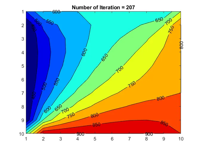
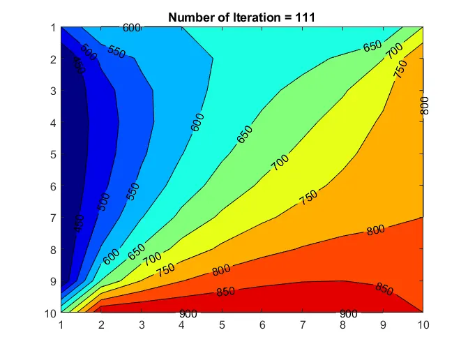
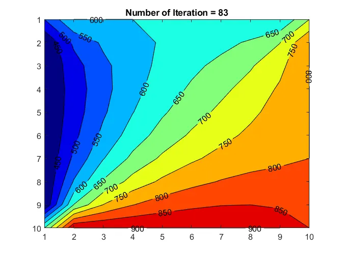
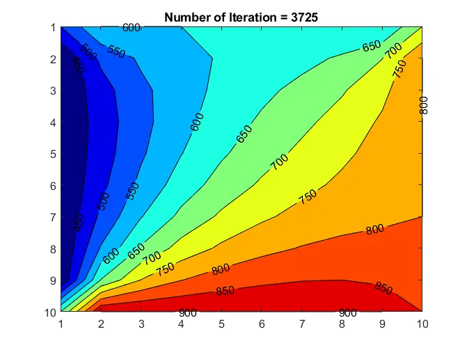
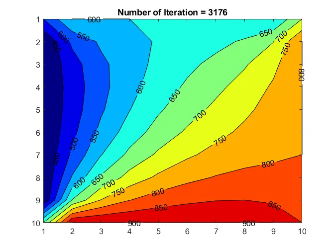
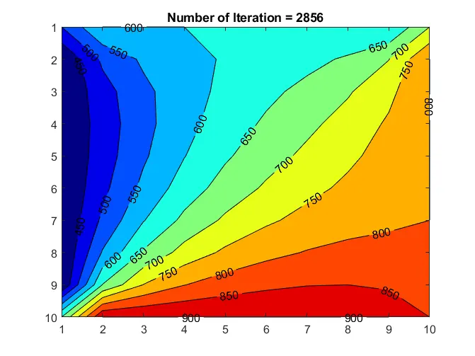
From the above iterative calculations, the following results are obtained. The results can be categorized on the basis of the accuracy of the solution and the number of iterations taken to achieve it.
The analytical calculation suggests that in the Jacobi method, the older temperature of the previous node is used to calculate the solution, thus reducing the accuracy and increasing the time to reach the same accurate solution.
In the Gauss-Seidel method, the solution is more accurate as the updated temperature of the previous node is used whose updated temperature is available, thus increasing the accuracy and reducing the time taken for simulation.
On the other hand, in the Successive Over Relaxation Method, the relaxation factor `omega` facilitates faster convergence.
a. Steady State
i.Jacobi Iterative Solver (Steady State)
ii Gauss-Seidel Method (Steady State)
iii SOR Iterative Solver (Steady State)
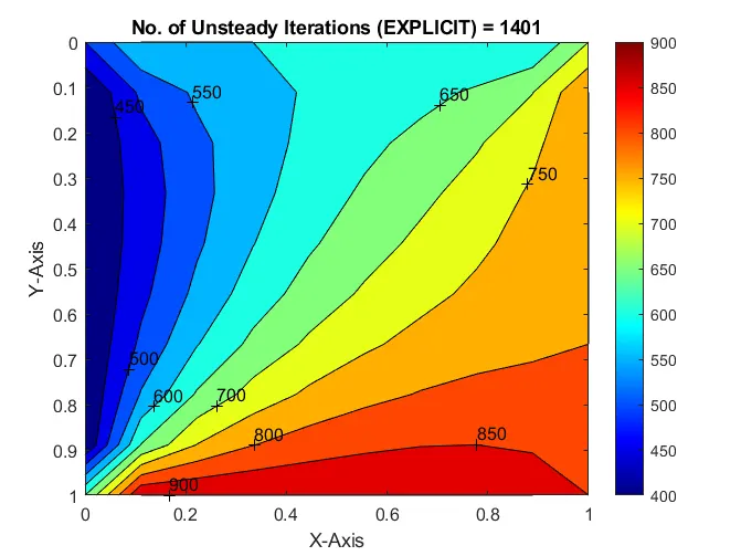
b. Unsteady State Explicit Method
c. Unsteady State Implicit Method
i. Jacobi Solver (Unsteady State)
ii. Gauss-Seidel Iterative Solvers (Steady State)
iii. SOR Iterative Solvers (Steady State)
Conclusion
The implicit method can be used to solve problems in which convergence is supposed to be achieved in less computation time as they are unconditionally stable. With the increase in time step size, the convergence rate is increased which leads to steady state solution with less no. of iterations.
The explicit method results are time accurate solutions as it is governed by stability criteria when not satisfied it leads to an unstable solution and requires more iterations to attain steady state.
But in the above code, the time step size remains constant which is calculated with respect to the stability criteria. Hence for this time step size the explicit scheme leads to a faster convergence rate and as the time step size is small the number of iterations increases for the implicit scheme which results in slower convergence rate.