Week 9 - FVM Literature Review

Finite Volume Method Literature Review

Objectives:

• To explain about Finite Volume Method (FVM) and how it differs from Finite Difference Method (FDM)
• To explain interpolation schemes and flux limiters in FVM

Some abbreviations:

FVM - Finite Volume Method

FDM - Finite Discrete Method

PDE - Partial Differential Equations

Finite Volume Method:

The Finite Volume method (FVM) is a numerical technique that transfers the Partial Differential Equation (PDE) representing the conservation laws over the differential volume into a discrete algebraic equation over the finite volumes.

FVM first discretizes the geometric domain into discrete non-overlapping elements or cells. The PDE is then discretized or transferred into discrete algebraic equations by integrating them over the finite volume. Then these discrete algebraic equations are then solved to compute the values of dependent variables for each of the elements.

Some characteristics of FVM:

• It is inherently conservative. In FVM, some terms in conservation equations are turned into face fluxes and evaluated at finite volume faces. The flux entering the given volume is the same as the flux exiting the volume. Hence FVM is conservative in nature.
• It can be formulated in the physical space on unstructured polygonal meshes.
• It is straightforward to implement a variety of boundary conditions in a non-invasive manner. Since the unknown variable is evaluated at the centroids of volume elements, not at their boundary faces.

The discretization procedure used in FVM is distinctive and involves two basic steps:

1. PDE --> Integrated PDE --> Balanced equation over an element (This involves changing the surface and volume integrals into discrete algebraic equations. The result is a Semi-discretized equation)
2. Interpolation schemes are chosen to approximate the variation of variables within the element, thus transforming the algebraic relations into algebraic equations.

In both the above steps, the selected approximation affects the accuracy and robustness of the resulting numerical.

Significant Differences between FVM and FDM:

• FVM - It is conserved across the entire domain.

FDM - It is easier to implement but we might face some problems with the conservation variables. More attention is required to study the boundary conditions.

• FVM - Dependent variable is stored at the center of the control volume.

FDM - Dependent variable is stored at each node.

• FVM - It uses the averages from the cell/finite volumes for the approximation of any function.

FDM - It uses the info only from the grid points for approximation of any function.

• FVM - It can be used for unstructured grids also.

FDM - It is mainly used for structured grids. It is difficult to implement FDM at curved boundaries. So for unstructured grids/complex geometries, we need to implement grid variables transformation. But it undergoes a more complex process.

Applying FVM to 1D Diffusion Problem (Heat transfer problem):

Let us see an example of implementing FVM to a 1D Diffusion problem (i.e, 1D Heat conduction problem)

Before going further, let's see the general transport equation for property `phi` and what this equation says, and how it relates to our 1D diffusion problem.

The general transport equation for the property `phi`:

`(del(rho phi))/(delt) + grad.(rhophiu) = grad.(|~gradphi) + S_phi` -----> (1)

where,

`|~` --> Diffusivity constant

`S` --> Source term

`phi` --> Transport property

Let us decompose equation (1) to understand its physical meaning as given below:

• `(del(rhophi))/(delt)` = Rate of increase of fluid element (Transient term).

• `grad.(rhophiu)` = Net rate of flow of `phi` out of the fluid element (Convection term).

• `grad.(|~gradphi)` = Rate of increase of `phi`due to diffusion (Diffusion term).

• `S_phi` = Rate of increase of `phi` due to source (Source term).

If we ignore the Transient term and Convective term from equation (1), the resulting is the general transport equation for the Diffusion problem.

The 1D Heat conduction problem is an example of a 1D Diffusion problem. Hence we can apply FVM to discretize the 1D Diffusion problem.

The 1D Steady state diffusion equation is given by,

`d/dx (|~(dphi)/dx) + S = 0` ----> (2)

`|~` - Diffusion constant

S - Source term

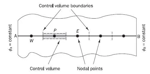
Step 1: Grid Generation

Divide the domain into discrete control volumes. We are targeting point P and nodes to the west and east are identified as W and E.

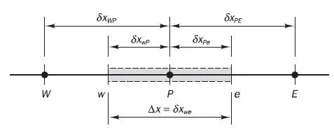
w & e - Boundary faces

`deltaX_(wp)` and `deltaX_(pe)` - Distance between boundary faces of control volume P and centroid of the control volume P

P, W, and E - Nodal points

`deltaX_(WP) and deltaX_(PE)` - Distance between Nodal point P and Nodal points W and E

Step 2: Discretization

In the FVM, we need to integrate the governing equation over a control volume to yield the discretized equation at its nodal point 'P'.

`int_(DeltaV) d/dx(|~(dphi)/dx) dV + int_(DeltaV) SdV = 0`

`(|~A(dphi)/dx)_e - (|~A(dphi)/dx)_w + bar SDeltaV = 0` ----> (3)

To derive equation (3), we need to know the values of `|~`(diffusion coefficient at boundary faces) and `((dphi)/dx)` at east (e) and west (w).

Since this is a uniform grid, we can estimate values of `|~_w and |~_e` by linearly interpolating.

`|~_w = (|~_W + |~_P)/2` ----> (4)

`|~_e = (|~_P + |~_E)/2` ----> (5)

The central differencing scheme is used to calculate `(dphi)/dx` at 'e' and 'w'.

`((dphi)/dx)_w = (phi_P - phi_w)/(deltaX_(WP))` ----> (6)

`((dphi)/dx)_e = (phi_E - phi_P)/(deltaX_(PE))` ----> (7)

Then for the Source term,

`bar SDeltaV = S_u + S_pphi_p` ----> (8)

Substituting equations (4), (5), (6), (7), and (8) in equation (3) we get,

`|~_e A_e ((phi_E - phi_P)/(deltaX_(PE))) - |~_w A_w ((phi_P - phi_W)/(deltaX_(WP))) + S_u + S_pphi_p = 0` ----> (9)

Making `phi_P` on LHS and `phi_W and phi_E` on RHS we get,

`[ ((|~_e A_e)/(deltaX_(PE))) + ((|~_w A_w )/(deltaX_(WP))) - S_p]phi_p = ((|~_w A_w )/(deltaX_(WP)))phi_W + ((|~_e A_e)/(deltaX_(PE)))phi_E + S_u` ----> (10)

Representing the coefficient of:

• `phi_P` as `a_P`
• `phi_W` as `a_W`
• `phi_E` as `a_E`

Then equation (10) becomes,

`a_P phi_P = a_Wphi_W+a_Ephi_E+S_u` ----> (11)

where,

`a_w = (|~_w A_w)/(deltaX)_(WP)`

`a_e = (|~_e A_e)/(deltaX)_(PE)`

`a_p = a_w+a_e-S_p`

Step 3: Solution of Equation

The discretized equation of the form (11) must be set up at each nodal point to solve the problem.

For control volumes adjacent to domain boundaries, the general discretized equation (11) is modified to incorporate boundary conditions.

The resulting system of equations (Linear Algebraic Equation) is then solved to obtain the distribution of property `phi` at each nodal point.

An example of a simple diffusion problem is the 1D Heat conduction problem. Where `phi` is replaced with the temperature `T` and `|~` is replaced with the Thermal diffusivity `alpha`.

Need for Interpolation schemes and Flux limiters in FVM

For the diffusion problems, the Central Differencing discretization schemes (CDS) might be worked well and produced stable and accurate solutions. But for the convection-diffusion problems, the CDS can no longer produce stable and accurate solutions. Hence the failure of CDS scheme is seen.

The failure is because of the `F/D` ratio is very high i.e., 5.

`F/D` ratio is nothing but the Peclet number `(F/D = (rhou)/(|~/(deltax)))`

In simple terms, we can say when we discretize the domain into less number grid points (for e.g. 5 grid points/elemental cells). The F/D ratio will go higher which leads to unstable solutions producing some wiggles or oscillations in the flux at the boundary faces where the result is physically unrealistic.

In contrast, let us discretize the same domain into 20 grid points/elemental cells (instead of 5) i.e., refining the mesh or making the mesh finer. Now the F/D ratio reduces to 1.25. The reduction in the F/D ratio results in stable and accurate solutions (no wiggles or oscillations).

But the problem is, in theory, the numerical simulations of infinitely large numbers of fine cells are possible. In practice, these many computational cells require more computational efforts.

Hence, most of the time we will be going with a small number of finite cells to perform simulations. So, in order to produce physically realistic results with a small number of finite cells/elemental cells, we need to depend on some interpolation schemes or discretization processes.

The following are some interpolation schemes available in FVM to address the aforementioned problem:

• Upwind Differencing Scheme (UDS)
• Linear Upwind Differencing scheme (LUD)
• Hybrid Differencing Scheme (HDS)
• Power law Scheme
• Quadratic Upwind Differencing Scheme (QUICK)
• Total Variation Diminishing Scheme (TVD)

References:

[1] H K Versteeg and W Malalasekera "An Introduction to Computational Fluid Dynamics THE FINITE VOLUME METHOD"

[2] F. Moukalled, L. Mangani, and M. Darwish "The Finite Volume Method in Computational Fluid Dynamics An Advanced Introduction with OpenFOAM® and Matlab®"

[3] Suhas V. and Patankar "Numerical Heat Transfer and Fluid Flow"