Week 8 - Simulation of a backward facing step in OpenFOAM

Simulation of a backward facing step in OpenFOAM

Objectives:

• To simulate the incompressible-laminar-viscous flow through the backward facing step geometry using OpenFOAM for the below cases:
  • CASE 1: Without the Grading factor
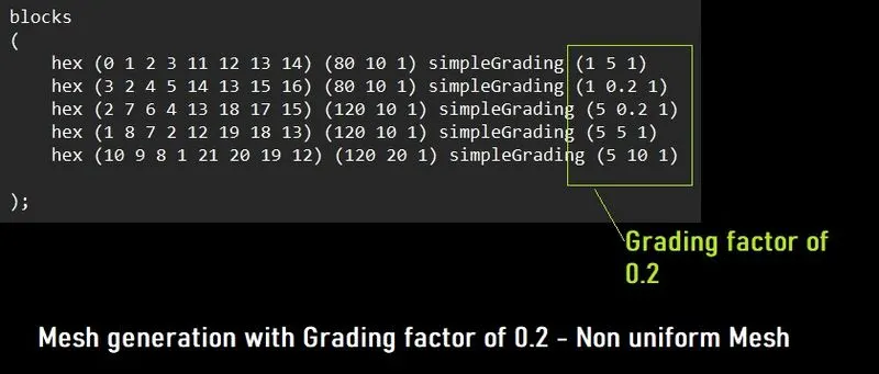
  • CASE 2: With the Grading factor (0.2)
• To plot the velocity plot at length 0.085 m from inlet of the geometry for both the cases.
• To explain the importance of Grading factor/Expansion ratio in mesh generation.

1. Introduction

In this project we need to simulate the incompressible-laminar-viscous flow through a backward facing step geometry. It is a 2D simulation where flow quantities along z direction is not considered.

The flow is considered to be incompressible when there is no change in density with respect to time through out the flow domain.

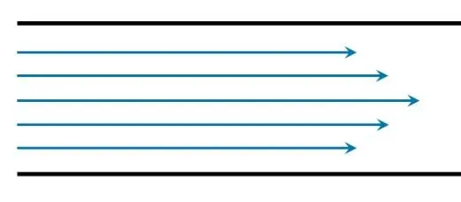
The flow is considered to be laminar when the streamlines are parallel to each other. Fluid moves slowly and is highly viscous.

In OpenFOAM, there are some dedicated solvers available for different kinds of flow problems. We need to decide a solver to be taken for our flow problem.

IcoFoam solver is responsible for undertaking the incompressible and laminar flow problems.

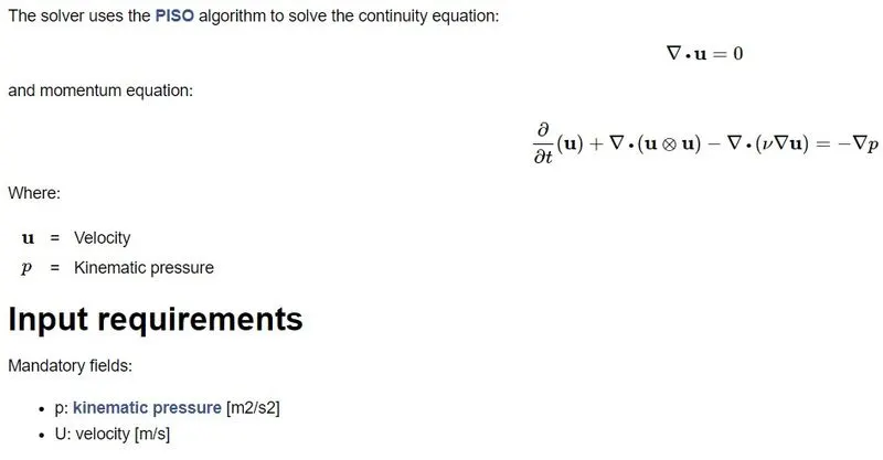
We need to take the corresponding case file from the OpenFOAM tutorials which solves the incompressible, laminar flow problems.

OpenFOAM Tutorial --> cavity [This case file has the icoFoam solver which solves incompressible and laminar flow problems]

The simulation has to be done to the below given geometry:

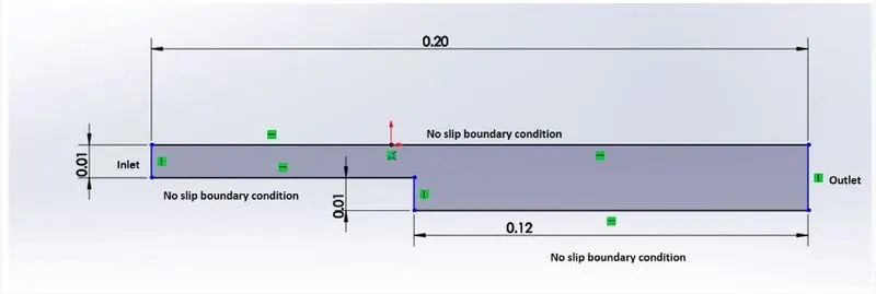
We need to copy the cavity case folder from the OpenFOAM tutorial and save it locally to modify the files.

Before proceeding further for the geometry creation, we need to understand the organisation and structure of a case folder. For e.g. Cavity case.

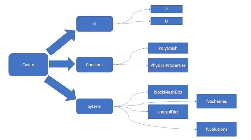
Copying a Case folder from the OpenFOAM tutorial

As mentioned earlier, we have decided to use icoFoam solver for this project. Hence the case folder corresponding to this solver is cavity case.

Steps to copy a case folder from OpenFOAM tutorial:

1. Open the Linux terminal via ubuntu.
2. Run the tut command in the terminal. Now the path changes to OpenFOAM Tutorials.
3. Run the ls command. It lists the variety of flow problems available in the OpenFOAM tutorial.
4. Run cd incompressible/ command to change the directory to incompressible flow folder.
5. Run ls command to display the list of solvers available in OpenFOAM tutorial for incompressible flow.
6. Run cd icoFoam/ command to change the directory to icoFoam solver folder.
7. Run ls command to display the list of projects available for this solver.
8. Run cd cavity/ command, then run ls command to display the list of cases available for this project and then run cd cavity/ again.
9. Run pwd command to display the current directory path and then copy this path.
10. Run run command. It will change to our home directory.
11. Run cp -ar <case path> . command to copy the case folder from the OpenFOAM tutorial to our home directory.
12. Now we can give whatever the name we wish for this case folder. For this project, I have created two copies of cavity case. One for CASE 1 (without grading factor) and another for CASE 2 (with grading factor).

2. Geometry Creation

This section describes procedures being followed to create a geometry for backward facing step.

1. From case folder (e.g. cavity_test), go to system --> blockMeshDict file.
2. Open the blockMeshDict file in Notepad or anyother text editor. You can also run gedit command to open the blockMeshDict file in Ubuntu's text editor.
3. Dimensions of the domain are:
4. OpenFOAM allows to create geometry in 3D cartesian coordinates system using vertices.
5. Let us consider creating the geometry using 5 blocks as shown below:
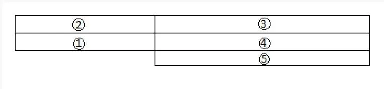
6. Let us start indexing the vertices for the blocks created. Since OpenFOAM uses C++ programming, we start indexing from '0'.
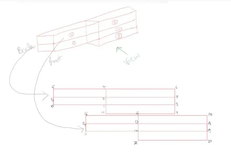
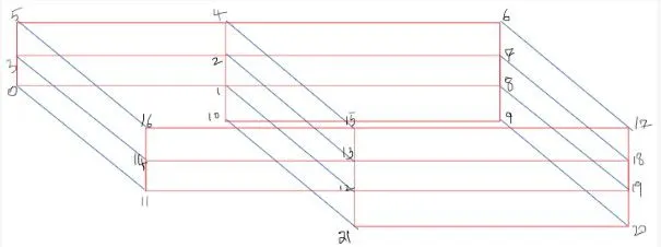
7. Open the blockMeshDict file. In the vertices dictionary, the following values are specified:
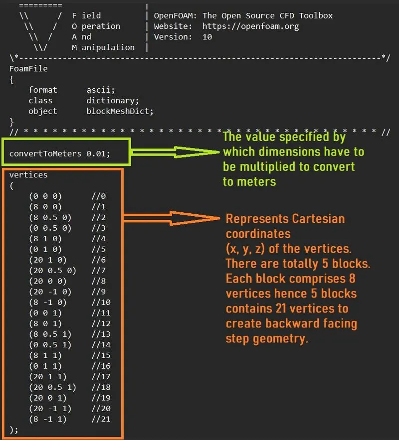
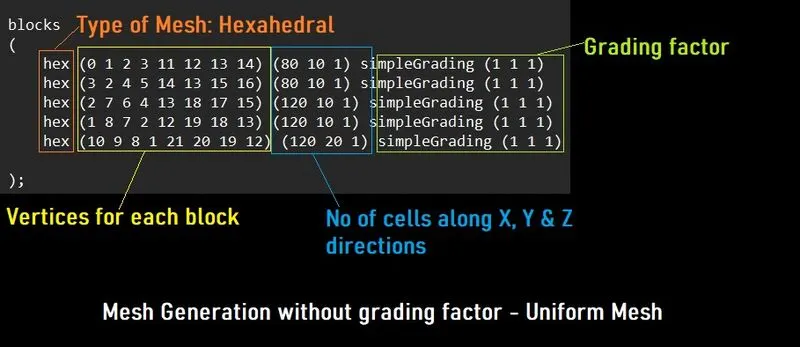
8. In the blocks dictionary,
   • CASE 1: Without grading factor
   • CASE 2: With Grading factor 0.2
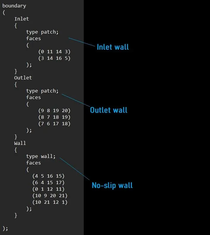
9. In the boundary dictionary, the values for inlet, outlet and walls are specified as given below:
10. Then mergePatchPairs dictionary is created and left empty inside. This dictionary is responsible for merging the above created blocks and patches (such as inlet, outlet and walls).
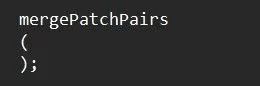
11. Save the file for both the cases (CASE 1 and CASE 2).

3. Mesh Generation

1. Now come to Ubuntu terminal, run blockMesh command to generate the mesh and run checkMesh command to verify the mesh has been created correctly without any error.
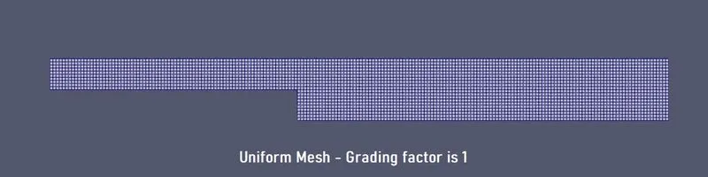
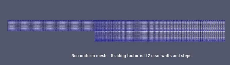
2. Run touch cavity_test.foam for CASE 2 (and touch cavity_test2.foam for CASE 1) in the terminal to view the generated mesh. The generated mesh for both cases are as follows:

4. Initial and Boundary Conditions

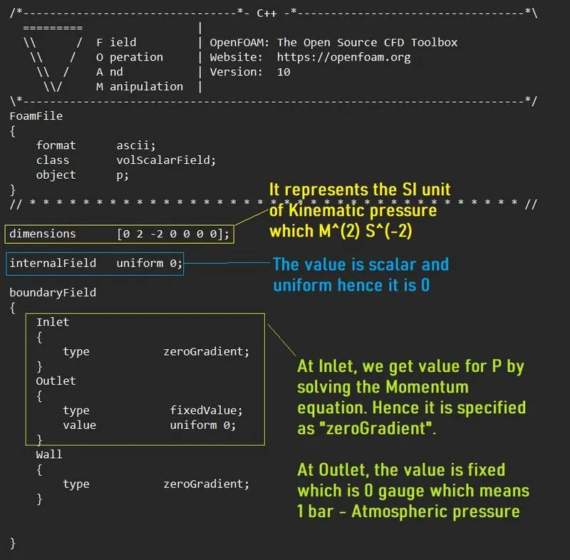
Now we need to specify the initial and bundary conditions such as

• Kinematic Pressure (p) and Velocity (U) at inlet and outlet at time `t = 0` --> P and U file
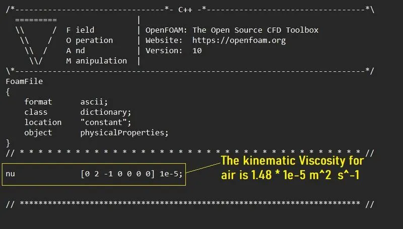
• Transport properties which is the kinematic Viscosity `nu` --> physicalProperties file
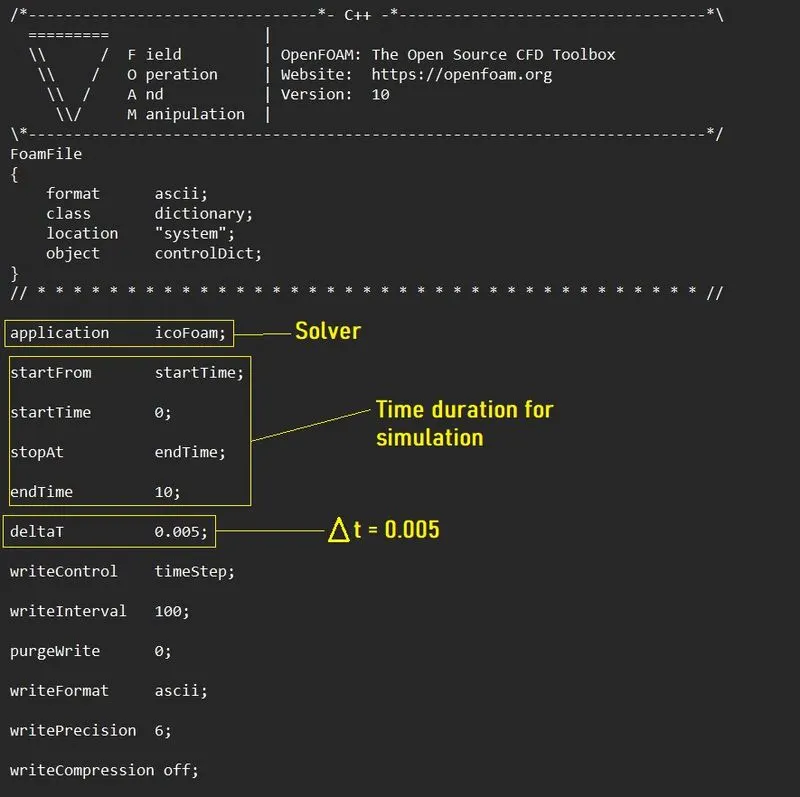
• Start time, End time and Simulation duration --> controlDict file

1. From case folder, go to 0 --> P file:

2. Then open the U file:

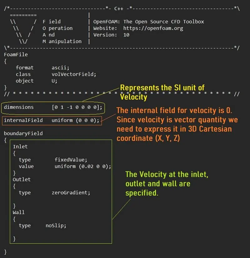
3. Then go to constant --> physicalProperties file, kinematic viscosity is taken as constant through out the domain.

4. And finally go to system --> controlDict file

5. Save all the files.

5. Running the icoFoam solver

Now come to Ubuntu Terminal and run the icoFoam solver.

Solver ran for 10 sec and ends

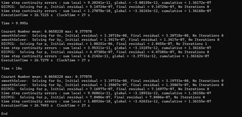
Here we could see the continuity and momentum equation is solved at each time step for pressure and velocity.

In Linux, we can solve this kind of problems and get output in terms of raw data.

Hence we need data visualization tool to view the simulation and plot the result.

6. Post-processing using Paraview

The output we get from running the icoFoam solver in OpenFOAM can be visualized in Paraview.

1. In OpenFOAM, simply run the command touch cavity_test.foam.
2. Paraview opens. Click Apply button.

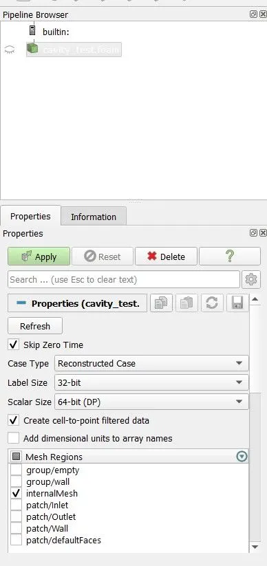
CASE 1: Without the grading factor - Uniform mesh

Uniform Mesh:

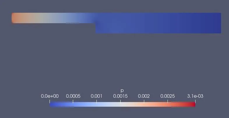
Pressure:

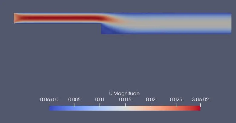
Velocity:

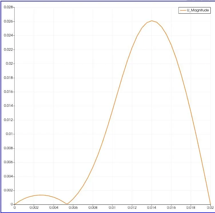
Velocity Plot at length 0.085 from the inlet:

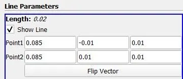
To plot the velocity at length 0.085 from the inlet,

1. Go to Filters menu --> Data Analysis --> Plot Over Line.
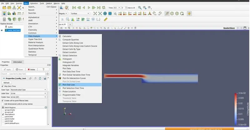
2. Set the length at which we need to visualize the velocity plot.

CASE 2: With Grading factor 0.2 - Non uniform mesh

Non uniform Mesh:

Pressure:

Velocity:

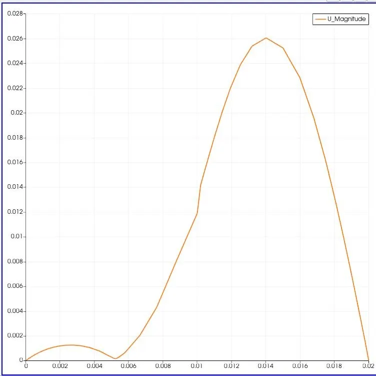
Velocity Plot at length 0.085 from the inlet:

7. Conclusion:

Comparison of the result for both the cases (CASE 1 & CASE 2):

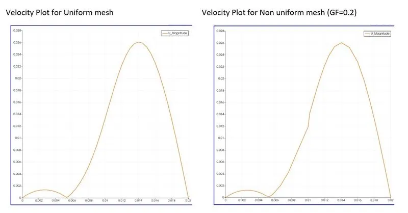
By comparing, we come to know that plot with grading factor (GF) 1 seems to be more accurate than the plot with GF 0.2.

Because for mesh with GF 0.2 where the mesh is not uniform disrupting our output result. On the other hand, flow quantities are very well captured at mesh near the walls. This is one of great advantage of grading the mesh.

Mesh needs to be finer in order to capture the flow properties with better accuracy. Hence the uniform mesh (GF=1) provides better result.