Week 7 - Simulation of a 1D Supersonic nozzle flow simulation using Macormack Method
Simulation of a 1D Supersonic nozzle flow simulation using MacCormack Method
Objective:
To simulate the isentropic flow through a quasi 1D subsonic-supersonic nozzle. The basic governing equation for quasi 1D nozzle flow is derived for both conservative and non-conservative form by implemeting the MacCormack's technique using MATLAB.
Problem Statement:
We need to determine the steady-state distribution for the flow-field variables and investigate the difference between the two forms of governing equations by comparing their solutions.
We need to show the following plots/results:
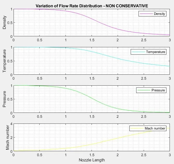
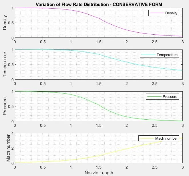
- Steady-state distribution of primitive variables inside the nozzle.
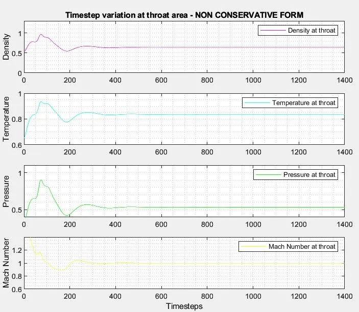
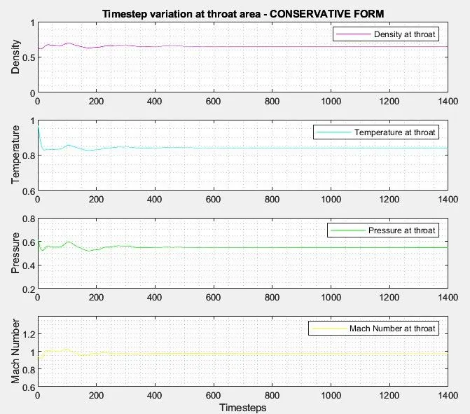
- Time-wise variation of the primitive variables.
- Variation of Mass flow rate distribution inside the nozzle at different time steps during the time-marching process.
- Comparison of Normalized mass flow rate distributions of both forms.
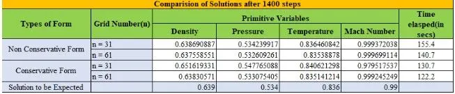
- Perform a grid independence test on the solution and expain all our findings.
I. Introduction
Let us consider the steady, isentropic flow through a convergent-divergent nozzle as given in the image below.
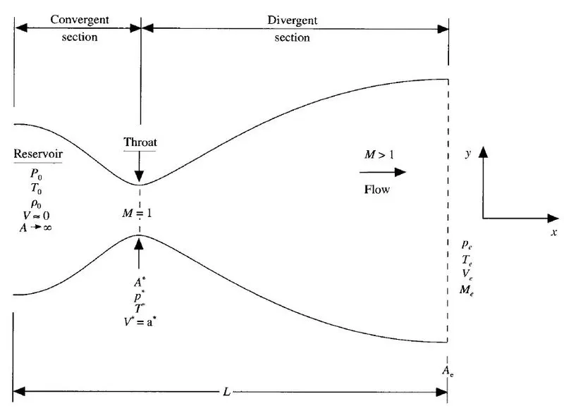
At the nozzle inlet, flow comes from a reservoir where the pressure, temperature and velocity are `p_o`, `T_o` and `(V-> 0)` respectively.
At the nozzle outlet, the flow expands isentropically (Adiabatic and reversible) to supersonic speed where the pressure, temperature and velocity are `p_e`, `T_e` and `V_e` respectively.
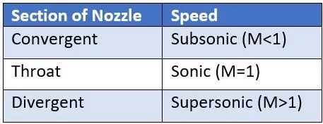
Let us assume that the flow properties `(p,V, T, rho, M)` vary only in x direction. Hence this flow is defined as Quasi 1D flow.
MacCormack Technique:
The CFD technique employed in this project is the MacCormack method which is the explicit, time-marching, finite difference solution for quasi 1D nozzle flow. It is second order accurate in both space and time.
The MacCormack method uses the forward differencing on predictor steps and backward differencing on the corrector steps to carry out the time marching solution.
Conservation and Non-conservation form:
There is a significance of the conservation versus the non-conservation form of the governing flow equations.
The conservation form of the equations is obtained directly from a control volume which is fixed in space rather than moving. When the volume is fixed in space, we are concerned with the flux of mass, momentum and energy into and out of the control volume. In this case, flux themselves become important dependent variables in the equations rather than just the primitive variables `(rho, p, V, T)`.
Theoretically, either form of the equation is a suitable representation of the fundamental physical principle of mass conservation, momentum conservation and energy conservation. However in CFD, there are some good numerical reason to use one form or the other form for the solution of certain flow parameters.
II. The Setup
This section comprises of the following three sub-sections:
- Governing equations
- Non-conservative form
- Conservative form
- The finite difference expressions pertaining to MacCormack's technique
- Non-conservative form
- Conservative form
- Other details for numerical simulation - Time step, Initial conditions, Boundary conditions.
- Non-conservative form
- Conservative form
II.A. Governing Equations
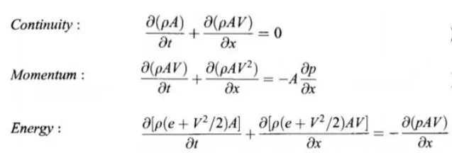
The governing equations for unsteady, inviscid, isentropic, quasi-1D nozzle nozzle flow is written in both non-conservative and conservative forms.
II.A.1 Non-conservative form
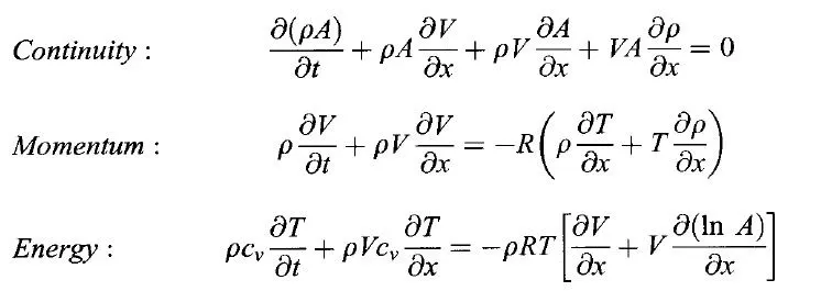
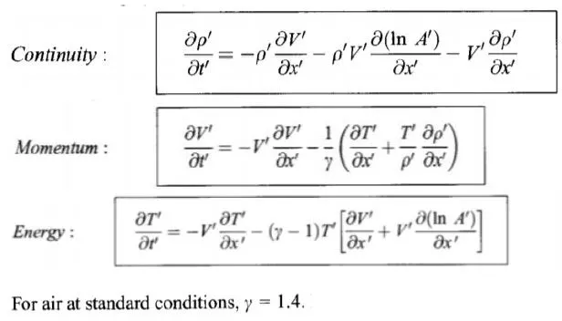
The above three equations are ready to setup our numerical solution. These are written in dimensional variable. However, for the nozzle floe simulation, the flow field variables are written in non-dimensional variables and the values varies between 0 and 1 which is an aesthetic advantage when presenting the result.
so rewritting the governing equations in non-dimensional form:
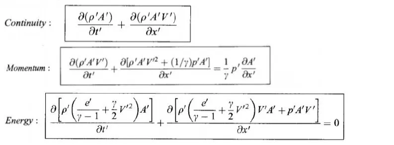
II.A.2 Conservative form
Rewritting the governing equations in non-dimensional form:
II.B. Finite Difference Equations pertaining to MacCormack's Technique
To implement the finite difference solution, we divide the x-axis along the nozzle into the number of discrete grid points as given in the image below:
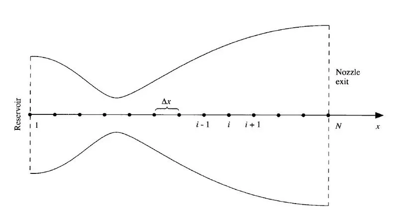
Point 1 is assumed to be in the reservoir/nozzle inlet.
Point N is assumed to be at the nozzle exit.
MacCormack techinque is a predictor-corrector method. In the time marching approach, the flow field variables at time t=0 is known and we use the difference equations to solve explicitly for those flow field variables at time t=`t+Deltat`
II.B.1 Non-conservative form
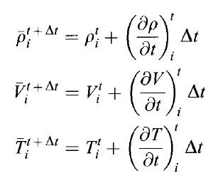
Predictor Step:
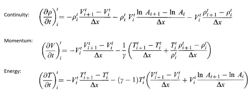
We can obtain the predicted values of `rho, V, and T` as given below:
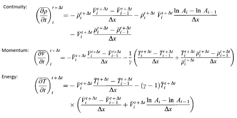
Corrector Step:
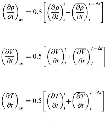
Calculating the average time derivative:
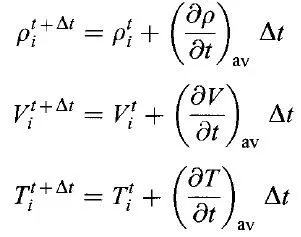
Corrected values of flow field variables at time `t = t+Deltat`:
II.B.2 Conservative form
The Conservative form of equations for the quasi 1D flow can be expressed in generic forms. Hence defining the elements of Solution vector U, the Flux vector F, Source term J.
First we need to find values for Solution vectors (`U_1, U_2, U_3`) using the primitive variables (`rho, V, T`) as given below:
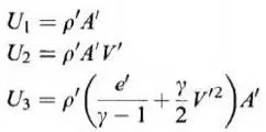
Next, using the values of solution vectors `U_1, U_2, U_3` we can find values for Flux terms`F_1, F_2, F_3`. Note that the instabilities are encountered when flux terms are constructed in terms of primitive variables. So, to attain a stable solution, constructing the flux terms with solution terms is more preferrable. However in theoretical basis, there is no big difference.
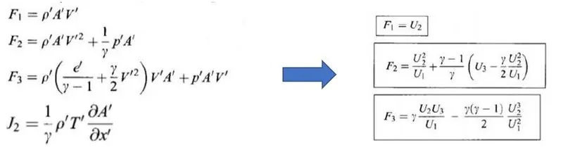
The final governing equation for unsteady, quasi 1D nozzle flow in conservative form is given by,
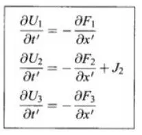
Predictor Step:
`((delU_1)/(delt))_i^t = -[F_(1(i+1)) - F_(1i)]/(Deltax)`
`((delU_2)/(delt))_i^t = -[F_(2(i+1)) - F_(2i])/(Deltax) + J_2`
`((delU_3)/(delt))_i^t = -[F_(3(i+1)) - F_(3i)]/(Deltax)`
We can obtain the predicted values of Solution terms (`U_1, U_2, U_3`)
`barU1_i^(t+Deltat) = U1_i^t + ((delU_1)/(delt))_i^t`
`barU2_i^(t+Deltat) = U2_i^t + ((delU_2)/(delt))_i^t`
`barU3_i^(t+Deltat) = U3_i^t + ((delU_3)/(delt))_i^t`
And obtain the predicted values of Flux terms (`F_1,F_2,F_3`) using the predicted values of Solution terms (`barU_1, barU_2, barU_3`). Then substitute these predicted values (both solution terms and flux terms) in the corrector step.
Corrector Step:
`((delbarU_1)/(delt))_i^(t +Deltat)= -[barF_(1i) - barF_(1(i-1))]/(Deltax)`
`((delbarU_2)/(delt))_i^(t +Deltat)= -[barF_(2i) - barF_(2(i-1))]/(Deltax)`
`((delbarU_3)/(delt))_i^(t +Deltat)= -[barF_(3i) - barF_(3(i-1))]/(Deltax)`
Calculating the average time derivative:
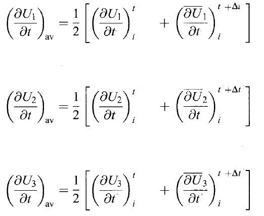
Corrected values of flow field variables at time `t = t+Deltat`:
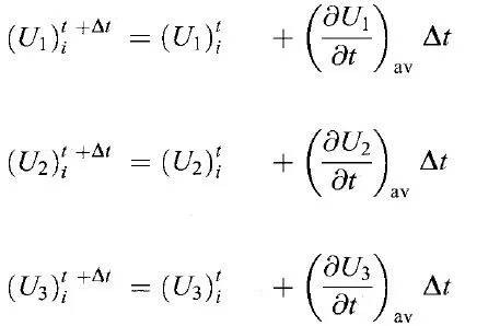
Finally, using the values of solution vectors (`U_1,U_2,U_3`) at `t + Deltat`, the primitive variables (`rho,V,T`) at `t + Deltat` can be calculated.
II.C. Other Details for Numerical Simulation - Time Step, Initial Conditions and Boundary Conditions
II.C.1 Time Step Calculation
Non-Conservative Form
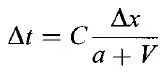
C - Courant Number. It is the simple stability analysis for linear hyberbolic equations. It should be `C<=1` for an explicit numerical solution to be stable.
V - Local flow velocity
a - Local speed of sound
Conservative Form
Same as non-conservative form.
II.C.2 Initial Conditions
Non-Conservative Form
In quasi 1D flow, all the flow properties changes with respect to x-direction only. Hence at time t=0,
Area of Nozzle `A = A(x) = 1 + 2.2(x-1.5)^2` `0<=x<=3`
`rho = 1-0.3146x`
`T = 1-0.2314x`
`V = (0.1+1.09x)sqrtT`
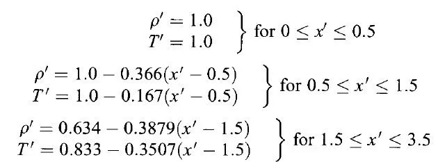
Conservative Form
Area of Nozzle remains same as non-conservative form.
II.C.3 Boundary Conditions
It is noted that unsteady, inviscid flow is governed by hyperbolic equations. For hyperbolic equations, there exists two real characteristic lines through point 1 and N.
Grid points 1 and N represent the two boundary points on x-axis. Where point 1 is inflow boundary and point N is outflow boundary.
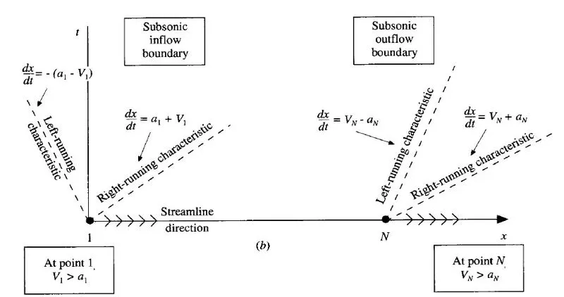
At point 1 (inflow boundary), one characteristic line propagates out of the domain and one propagates into the domain. Which means one variable is allowed to float and other variables to be stipulated (specified exactly). Hence we choose Velocity variable to float and other variables (`rho, T`) to be stipulated.
At point N (outflow boundary), both the two characteristic lines propagates out of the domain. Which means all variables are allowed to float.
The numerical implementation for this boundary condition is as follows:
Non-Conservative Form
Inflow Boundary:
`rho_1 = 1` and `T_1 = 1`
For floating variable V changes with respect to time. Hence we use linear extrapolation to find V at point 1 using points 2 and 3.
By linearly extrapolating, we get `V_1 = 2V_2-V_3`
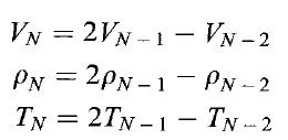
Outflow Boundary:
All variables are allowed to float.
Conservative Form
Inflow Boundary:
Same as in non-conservative form where two flow properties are held fixed and one flow property is allowed to float.
As we know that for conservative form, we express flow field variables in generic form i.e., `U_1, U_2, U_3`
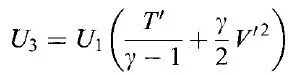
`U_1 = rho_1A_1` if `rho_1` is held fixed which is 1. Hence `U_1 = 1`
`U_2 = rho_1A_1V_1` where `V_1` is allowed to float. Hence `U_(2(i=1)) = 2U_(2(i=2)) - U_(2(i=3))`
Outflow Boundary:
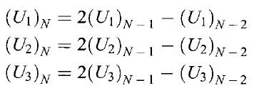
All the flow properties are allowed to float. Hence,
III. Simulation in MATLAB
The simulation of 1D supersonic nozzle flow is performed using MATLAB by implementing all the above theoretical concepts such as governing equations, MacCormack's technique etc.,
The algorithm for this simulation contains:
- Main Program
- Function for Non-conservative form
- Function for Conservative form
When executing the main program, it calls the corresponding functions to perform the necessary calculations and provide results (plots).
III.A. Main Program
clear all
close all
clc

%SOLVING QUASI 1D SUPERSONIC NOZZLE FLOW EQUATIONS

%INPUT PARAMETERS
%No. of grid points
n = 31;

gamma = 1.4;
x = linspace(0,3,n);
dx = x(2) - x(1);

%No. of time step
nt = 1400;

%Courant Number
C = 0.5;


%FUNCTION FOR NON CONSERVATIVE FORM
tic;
[Mass_flow_rate_NC, Pressure_NC, Mach_number_NC, rho_NC, v_NC, T_NC, rho_throat_NC, v_throat_NC, T_throat_NC, Mass_flow_rate_throat_NC, Pressure_throat_NC, Mach_number_throat_NC] = non_conservative_form(x, dx, n, gamma, nt, C);
Time_elapsed_NC = toc;
fprintf('Time Elasped for Non Conservative form: %0.4f', Time_elapsed_NC);
hold on

%PLOTTING
%Timestep variation of properties at throat area in Non Conservative form
figure(2)

%Density
subplot(4,1,1)
plot(linspace(1,nt,nt),rho_throat_NC,'color','m')
ylabel('Density')
legend({'Density at throat'})
axis([0 1400 0 1.3])
grid minor
title('Timestep variation at throat area - NON CONSERVATIVE FORM')

%Temperature
subplot(4,1,2)
plot(linspace(1,nt,nt),T_throat_NC,'color','c')
ylabel('Temperature')
legend({'Temperature at throat'})
axis([0 1400 0.6 1])
grid minor

%Pressure
subplot(4,1,3)
plot(linspace(1,nt,nt),Pressure_throat_NC,'color','g')
ylabel('Pressure')
legend({'Pressure at throat'})
axis([0 1400 0.4 1.1])
grid minor

%Mach Number
subplot(4,1,4)
plot(linspace(1,nt,nt),Mach_number_throat_NC,'color','y')
xlabel('Timesteps')
ylabel('Mach Number')
legend({'Mach Number at throat'})
axis([0 1400 0.6 1.4])
grid minor


%Steady state simulation for primitve values for Non Conservative form
figure(3);
%Density

subplot(4,1,1);
plot(x,rho_NC,'color','m')
ylabel('Density')
legend({'Density'})
axis([0 3 0 1])
grid minor
title('Variation of Flow Rate Distribution - NON CONSERVATIVE')

%Temperature
subplot(4,1,2);
plot(x,T_NC,'color','c')
ylabel('Temperature')
legend({'Temperature'})
axis([0 3 0 1])
grid minor

%Pressure
subplot(4,1,3);
plot(x,Pressure_NC,'color','g')
ylabel('Pressure')
legend({'Pressure'})
axis([0 3 0 1])
grid minor

%Mach number
subplot(4,1,4);
plot(x,Mach_number_NC,'color','y')
xlabel('Nozzle Length')
ylabel('Mach number')
legend({'Mach number'})
axis([0 3 0 4])
grid minor

%FUNCTION FOR CONSERVATIVE FORM
tic;
[Mass_flow_rate_C, Pressure_C, Mach_number_C, rho_C, v_C, T_C, rho_throat_C, v_throat_C, T_throat_C, Mass_flow_rate_throat_C, Pressure_throat_C, Mach_number_throat_C] = conservative_form(x, dx, n, gamma, nt, C);
Time_elasped_C = toc;
fprintf('Time Elasped for Conservative form: %0.4f', Time_elasped_C);

%PLOTTING
%Timestep variation of properties at throat area in Conservative form
figure(5)

%Density
subplot(4,1,1)
plot(rho_throat_C,'color','m')
ylabel('Density')
legend({'Density at throat'})
axis([0 1400 0 1])
grid minor
title('Timestep variation at throat area - CONSERVATIVE FORM')

%Temperature
subplot(4,1,2)
plot(T_throat_C,'color','c')
ylabel('Temperature')
legend({'Temperature at throat'})
axis([0 1400 0.6 1])
grid minor

%Pressure
subplot(4,1,3)
plot(Pressure_throat_C,'color','g')
ylabel('Pressure')
legend({'Pressure at throat'})
axis([0 1400 0.2 0.8])
grid minor

%Mach Number
subplot(4,1,4)
plot(Mach_number_throat_C,'color','y')
xlabel('Timesteps')
ylabel('Mach Number')
legend({'Mach Number at throat'})
axis([0 1400 0.6 1.4])
grid minor


%Steady state simulation for primitve values for Non Conservative form
figure(6);

%Density
subplot(4,1,1);
plot(x,rho_C,'color','m')
ylabel('Density')
legend({'Density'})
axis([0 3 0 1])
grid minor
title('Variation of Flow Rate Distribution - CONSERVATIVE FORM')

%Temperature
subplot(4,1,2);
plot(x,T_C,'color','c')
ylabel('Temperature')
legend({'Temperature'})
axis([0 3 0 1])
grid minor

%Pressure
subplot(4,1,3);
plot(x,Pressure_C,'color','g')
ylabel('Pressure')
legend({'Pressure'})
axis([0 3 0 1])
grid minor

%Mach number
subplot(4,1,4);
plot(x,Mach_number_C,'color','y')
xlabel('Nozzle Length')
ylabel('Mach number')
legend({'Mach number'})
axis([0 3 0 4])
grid minor


%COMPARISON PLOT of Normalized Mass Flow Rate of both forms
figure(7)
hold on
plot(x,Mass_flow_rate_NC,'r','linewidth',1.25)
hold on
plot(x,Mass_flow_rate_C,'b','linewidth',1.25)
hold on
grid on

legend('Non Conservative','Conservative')
xlabel('Length of the Domain')
ylabel('Mass Flow Rate')
title('Comparison of Normalized Mass Flow Rate of both forms')
Code Explanation:
- The input parameters such as Number of grid points (n), Specific heat ratio of air (`gamma`), Grid points (x), Distance of grid points (`Deltax`), Number of time steps (nt), and Courant Number (C) are specified.
- A function call is made for the Non-conservative form. Simultaneously, tic and toc function is written to evaluate the time taken by the non-conservative form function to process and provide outputs.
- Plotting for Timestep variation of properties (`rho,T, P,M`) at throat area of Non-conservative form code is written.
- Plotting for steady state simulation for primitve values (`rho,T, P,M`) of Non-conservative form code is written.
- A function call is made for the Conservative form. Simultaneously, tic and toc function is written to evaluate the time taken by the conservative form function to process and provide outputs.
- Plotting for Timestep variation of properties (`rho,T, P,M`) at throat area of Conservative form code is written.
- Plotting for steady state simulation for primitve values (`rho,T, P,M`) of Conservative form code is written.
- Plotting for COMPARISON PLOT of Normalized Mass Flow Rate of both forms code is written.
%Function for Non-Conservative form

function [Mass_flow_rate_NC, Pressure_NC, Mach_number_NC, rho_NC, v_NC, T_NC, rho_throat_NC, v_throat_NC, T_throat_NC, Mass_flow_rate_throat_NC, Pressure_throat_NC, Mach_number_throat_NC] = non_conservative_form(x, dx, n, gamma, nt, C)

%Intial boundary conditions
rho_NC = 1 - 0.3146*x;
T_NC = 1 - 0.2341*x;
v_NC = (0.1 + 1.09*x).*T_NC.^0.5;

%Area & Throat profiles
a = 1 + 2.2*(x - 1.5).^2;
throat = find(a==1);


%Outer Time Loop
for k = 1:nt

    %Time-step control
    dt = min(C.*dx./(sqrt(T_NC) + v_NC));

    %Saving a copy of Old Values
    rho_old = rho_NC;
    T_old = T_NC;
    v_old = v_NC;


    %Predictor Method
    for j = 2:n-1

        %Simplifying the Equation's spatial terms
        dv_dx = (v_NC(j + 1) - v_NC(j))/dx;
        drho_dx = (rho_NC(j + 1) - rho_NC(j))/dx;
        dT_dx = (T_NC(j + 1) - T_NC(j))/dx;
        dlog_a_dx = (log(a(j + 1)) - log(a(j)))/dx;

        %Continuity Equation
        drho_dt_P(j) = -rho_NC(j)*dv_dx - rho_NC(j)*v_NC(j)*dlog_a_dx - v_NC(j)*drho_dx;

        %Momentum Equation
        dv_dt_P(j) = -v_NC(j)*dv_dx - (1/gamma)*(dT_dx + (T_NC(j)*drho_dx/rho_NC(j)));

        %Energy Equation
        dT_dt_P(j) = -v_NC(j)*dT_dx - (gamma - 1)*T_NC(j)*(dv_dx + v_NC(j)*dlog_a_dx);


        %Solution Update
        rho_NC(j) = rho_NC(j) + drho_dt_P(j)*dt;
        v_NC(j) = v_NC(j) + dv_dt_P(j)*dt;
        T_NC(j) = T_NC(j) + dT_dt_P(j)*dt;

    end


    %Corrector Method
    for j = 2:n-1

        %Simplifying the Equation's spatial terms
        dv_dx = (v_NC(j) - v_NC(j - 1))/dx;
        drho_dx = (rho_NC(j) - rho_NC(j - 1))/dx;
        dT_dx = (T_NC(j) - T_NC(j - 1))/dx;
        dlog_a_dx = (log(a(j)) - log(a(j - 1)))/dx;

        %Continuity Equation
        drho_dt_C(j) = - rho_NC(j)*dv_dx - rho_NC(j)*v_NC(j)*dlog_a_dx - v_NC(j)*drho_dx;

        %Momentum Equation
        dv_dt_C(j) = - v_NC(j)*dv_dx - (1/gamma)*(dT_dx + (T_NC(j)*drho_dx/rho_NC(j)));

        %Energy Equation
        dT_dt_C(j) = - v_NC(j)*dT_dx - (gamma - 1)*T_NC(j)*(dv_dx + v_NC(j)*dlog_a_dx);

    end

    %Compute Average Time derivative
    drho_dt = 0.5.*(drho_dt_P + drho_dt_C);
    dv_dt = 0.5.*(dv_dt_P + dv_dt_C);
    dT_dt = 0.5.*(dT_dt_P + dT_dt_C);

    %Final Solution Update
    for i = 2:n-1
        rho_NC(i) = rho_old(i) + drho_dt(i)*dt;
        v_NC(i) = v_old(i) + dv_dt(i)*dt;
        T_NC(i) = T_old(i) + dT_dt(i)*dt;

    end

    %Applying Boundary Conditions
    %At Inlet
    rho_NC(1) = 1;
    v_NC(1) = 2*v_NC(2) - v_NC(3);
    T_NC(1) = 1;

    %At Outlet
    rho_NC(n) = 2*rho_NC(n-1) - rho_NC(n - 2);
    v_NC(n) = 2*v_NC(n - 1) - v_NC(n - 2);
    T_NC(n) = 2*T_NC(n - 1) - T_NC(n - 2);


    %Defining Mass flow rate, Pressure and Mach number
    Mass_flow_rate_NC = rho_NC.*a.*v_NC;
    Pressure_NC = rho_NC.*T_NC;
    Mach_number_NC = (v_NC./sqrt(T_NC));

    %Calculating Variables at throat section
    rho_throat_NC(k) = rho_NC(throat);
    T_throat_NC(k) = T_NC(throat);
    v_throat_NC(k) = v_NC(throat);
    Mass_flow_rate_throat_NC(k) = Mass_flow_rate_NC(throat);
    Pressure_throat_NC(k) = Pressure_NC(throat);
    Mach_number_throat_NC(k) = Mach_number_NC(throat);


    %PLOTTING
    %Comparison of non-dimensional Mass flow rates at different time steps
    figure(1);
    if k == 50
       plot(x, Mass_flow_rate_NC, 'r', 'linewidth', 2);
       hold on
    elseif k == 100
       plot(x, Mass_flow_rate_NC, 'b', 'linewidth', 2);
       hold on
    elseif k == 200
       plot(x, Mass_flow_rate_NC, 'g', 'linewidth', 2);
       hold on
    elseif k == 400
       plot(x, Mass_flow_rate_NC, 'y', 'linewidth', 2);
       hold on
    elseif k == 800
       plot(x, Mass_flow_rate_NC, 'k', 'linewidth', 2);
       hold on
    end

    %Labelling
    title('Mass flow rates at different Timesteps - NON CONSERVATIVE FORM)')
    xlabel('Distance')
    ylabel('Mass flow rate')
    legend({'50^t^h Timestep','100^t^h Timestep','200^t^h Timestep','400^t^h Timestep','800^t^h Timestep'})
    axis([0 3 0 2])
    grid on

end

end
Code Explanation
- The function's input arguments (from the main program) and output arguments (to the main program) are specifed.
- Initial conditions of `Density(rho), Velocity( V), Temperature(T), Area(A)` at time t = 0 are specified.
- Time loop (from t=1 to t=1400) starts using the values initial conditions (`rho, V, T,A`) at time t=0:
- The time step `Deltat` is calculated. Here the Courant number (C) is taken as 0.5 which is the stability criteria for the explicit numerical solution.
- The primitive variables (`rho,V,T`) at time t=0 is saved for future purpose.
- Predictor method for internal grid points (point 2 to point n-1) loop starts:
- Before performing the calculation for solving the governing equation, the governing equation's spatial terms (on RHS) gets decomposed in finite difference form (forward differencing) to simplify the calculation.
- The basic governing equations (Continuity, Momentum and Energy) which is in the finite difference form (forward differencing) is solved.
- The predicted values are calculated and ready to pass into the Corrector method.
- Corrector method for internal grid points (point 2 to point n-1) loop starts:
- Before performing the calculation for solving the governing equation, the governing equation's spatial terms (on RHS) gets decomposed in finite difference form (backward differencing) to simplify the calculation.
- The basic governing equations (Continuity, Momentum and Energy) which is in the finite difference form (backward differencing) is solved.
- The average of time derivative which is obtained from predictor method and corrector method is evaluated.
- Final solution update is made for the internal grid points (from point 2 to point n-1) by the addition of the primitive variable in the previous time step (in this case, it is t=0) and the average time derivative of primitive variables which is obtained in the current time step (t=1).
- Applying the boundary conditions at inlet and outlet so that the flow field varaibles (or primitive variables) at point 1 and point N are calculated and passed onto the next time steps (i.e., t=2,.....,1400)
- Using the values obtained from the final solution update(`rho,V,T`), other flow field variables (Mass flow rate, Mach Number and Pressure at all the grid points) which are functions of `rho,V,T`are calculated
- Similarly, all these flow field variables (`rho,P,V,T`, Mass flow rate, Mach number) at throat section are calculated.
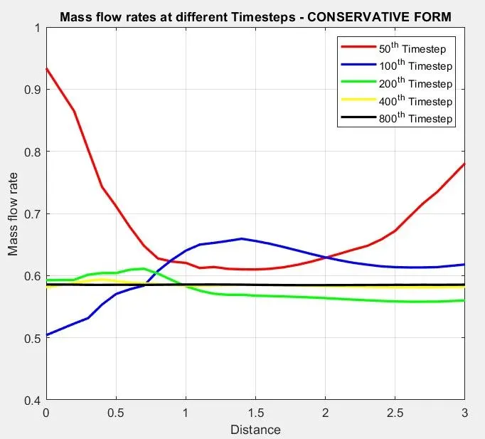
- With in these time loop (t = 1 to 1400), the obtained mass flow rate at different time steps (t = 50, 100, 200, 400 and 800) is plotted to show how the numerical solution reaches the steady state by increasing the number of time steps.
- Time loop ends.
III.C. Function for Conservative form
%Function for Conservative form

function [Mass_flow_rate_C, Pressure_C, Mach_number_C,  rho_C, v_C, T_C, rho_throat_C, v_throat_C, T_throat_C, Mass_flow_rate_throat_C, Pressure_throat_C, Mach_number_throat_C] = conservative_form(x, dx, n, gamma, nt, C)

%Determining Initial profile of Density and Temperature
for i = 1:n

    if (x(i) >= 0 && x(i) <= 0.5)
        rho_C(i) = 1;
        T_C(i) = 1;
    elseif (x(i) >= 0.5 && x(i) <= 1.5)
        rho_C(i) = 1 - 0.366*(x(i) - 0.5);
        T_C(i) = 1 - 0.167*(x(i) - 0.5);
    elseif (x(i) >= 1.5 && x(i) <= 3)
        rho_C(i) = 0.634 - 0.3879*(x(i) - 1.5);
        T_C(i) = 0.833 - 0.3507*(x(i) - 1.5);
    end

end

%Area & Throat profiles
a = 1 + 2.2*(x - 1.5).^2;
throat = find(a==1);

%Initial profile for Velocity and Pressure
v_C = 0.59./(rho_C.*a);
Pressure_C = rho_C.*T_C;

%Calculate the Initial Solution Vectors(U)
U1 = rho_C.*a;
U2 = rho_C.*a.*v_C;
U3 = rho_C.*a.*(T_C./(gamma - 1)) + ((gamma/2).*v_C.^2);


%Outer Time Loop
for k =1:nt

    %Time-step control
    dt = min(C.*dx./(sqrt(T_C) + v_C));

    %Saving a copy of Old Values
    U1_old = U1;
    U2_old = U2;
    U3_old = U3;

    %Calculating the Flux vector(F)
    F1 = U2;
    F2 = ((U2.^2)./U1) + ((gamma - 1)/gamma)*(U3 - (gamma/2)*((U2.^2)./U1));
    F3 = ((gamma*U2.*U3)./U1) - (gamma*(gamma - 1)*((U2.^3)./(2*U1.^2)));


    %Predictor Method
    for j = 2:n-1

        %Calculating the Source term(J)
        J2(j) = (1/gamma)*rho_C(j)*T_C(j)*((a(j + 1) - a(j))/dx);


        %Continuity Equation
        dU1_dt_P(j) = -((F1(j + 1) - F1(j))/dx);

        %Momentum Equation
        dU2_dt_P(j) = -((F2(j + 1) - F2(j))/dx) + J2(j);

        %Energy Equation
        dU3_dt_P(j) = -((F3(j + 1) - F3(j))/dx);


        %Updating New values
        U1(j) = U1(j) + dU1_dt_P(j)*dt;
        U2(j) = U2(j) + dU2_dt_P(j)*dt;
        U3(j) = U3(j) + dU3_dt_P(j)*dt;

    end

    %Updating Flux vectors
    F1 = U2;
    F2 = ((U2.^2)./U1) + ((gamma - 1)/gamma)*(U3 - ((gamma*0.5*(U2.^2))./(U1)));
    F3 = ((gamma*U2.*U3)./U1) - ((gamma*0.5*(gamma - 1)*(U2.^3))./(U1.^2));


    %Corrector Method
    for j = 2:n-1

        %Updating the Source term(J)
        J2(j) = (1/gamma)*rho_C(j)*T_C(j)*((a(j) - a(j - 1))/dx);

        %Simplifying the Equation's spatial terms
        dU1_dt_C(j) = -((F1(j) - F1(j - 1))/dx);
        dU2_dt_C(j) = -((F2(j) - F2(j - 1))/dx) + J2(j);
        dU3_dt_C(j) = -((F3(j) - F3(j - 1))/dx);

    end

    %Compute Average Time derivative
    dU1_dt = 0.5*(dU1_dt_P + dU1_dt_C);
    dU2_dt = 0.5*(dU2_dt_P + dU2_dt_C);
    dU3_dt = 0.5*(dU3_dt_P + dU3_dt_C);

    %Final Solution Update
    for i = 2:n-1
        U1(i) = U1_old(i) + dU1_dt(i)*dt;
        U2(i) = U2_old(i) + dU2_dt(i)*dt;
        U3(i) = U3_old(i) + dU3_dt(i)*dt;

    end


    %Applying Boundary Conditions
    %At Inlet
    U1(1) = rho_C(1)*a(1);
    U2(1) = 2*U2(2) - U2(3);

    v_C(1) = U2(1)./U1(1);
    U3(1) = U1(1)*((T_C(1)/(gamma - 1)) + ((gamma/2)*(v_C(1)).^2));

    %At Outlet
    U1(n) = 2*U1(n - 1) - U1(n - 2);
    U2(n) = 2*U2(n - 1) - U2(n - 2);
    U3(n) = 2*U3(n - 1) - U3(n - 2);

    %Final Primitive value update
    rho_C = U1./a;
    v_C = U2./U1;
    T_C = (gamma - 1)*((U3./U1 - (gamma/2)*(v_C).^2));

    %Defining Mass flow rate, Pressure and Mach number
    Mass_flow_rate_C = rho_C.*a.*v_C;
    Pressure_C = rho_C.*T_C;
    Mach_number_C = (v_C./sqrt(T_C));

    %Calculating Variables at throat section
    rho_throat_C(k) = rho_C(throat);
    T_throat_C(k) = T_C(throat);
    v_throat_C(k) = v_C(throat);
    Mass_flow_rate_throat_C(k) = Mass_flow_rate_C(throat);
    Pressure_throat_C(k) = Pressure_C(throat);
    Mach_number_throat_C(k) = Mach_number_C(throat);

    %PLOTTING
    %Comparison of non-dimensional Mass flow rates at different time steps
    figure(4)
    if k == 50
       plot(x, Mass_flow_rate_C, 'r', 'linewidth', 2);
       hold on
    elseif k == 100
       plot(x, Mass_flow_rate_C, 'b', 'linewidth', 2);
       hold on
    elseif k == 200
       plot(x, Mass_flow_rate_C, 'g', 'linewidth', 2);
       hold on
    elseif k == 400
       plot(x, Mass_flow_rate_C, 'y', 'linewidth', 2);
       hold on
    elseif k == 800
       plot(x, Mass_flow_rate_C, 'k', 'linewidth', 2);
       hold on
    end


    %Labelling
    title('Mass flow rates at different Timesteps - CONSERVATIVE FORM')
    xlabel('Distance')
    ylabel('Mass flow rate')
    legend({'50^t^h Timestep','100^t^h Timestep','200^t^h Timestep','400^t^h Timestep','800^t^h Timestep'})
    axis([0 3 0.4 1])
    grid on

end

end
Code Explanation
- The function's input arguments (from the main program) and output arguments (to the main program) are specifed.
- Initial conditions of `Density(rho), Velocity( V), Temperature(T), Area(A)` at time t = 0 are specified.
- The solution terms (`U_1,U_2,U_3`) is calculated using the primitive variables (`rho,V,T,`) at time t=0.
- Time loop (from t=1 to t=1400) starts using the values initial conditions (`rho, V, T,A`) at time t=0:
- The time step `Deltat` is calculated. Here the Courant number (C) is taken as 0.5 which is the stability criteria for the explicit numerical solution.
- The solution terms (`U_1,U_2,U_3`) at time t=0 is saved for future purpose.
- The Flux terms (`F_1,F_2,F_3`) values are calculated using the solution terms.
- Predictor method for internal grid points (point 2 to point n-1) loop starts:
- The basic governing equations (Continuity, Momentum and Energy) which is in generic forms is solved using the finite difference form (forward differencing).
- Updating the new values of solution terms at all the grid points (point 2 to point n-1).
- Flux terms get updated with the new values of solution terms at all the grid points.
- Corrector method for internal grid points (point 2 to point n-1) loop starts:
- The basic governing equations (Continuity, Momentum and Energy) which is in generic forms is solved using the finite difference form (backward differencing).
- The average of time derivative which is obtained from predictor method and corrector method is evaluated.
- Final solution update is made for the internal grid points (from point 2 to point n-1) by the addition of the solution terms in the previous time step (in this case, it is t=0) and the average time derivative of the solution terms which is obtained in the current time step (t=1).
- Applying the boundary conditions at inlet and outlet so that the solution terms at point 1 and point N are calculated and passed onto the next time steps (i.e., t=2,.....,1400).
- The final primitive variables (`rho, V, T, ) is calculated using the solution terms (`U_1,U_2,U_3`).
- Using the values obtained from the final solution update(`rho,V,T`), other flow field variables (Mass flow rate, Mach Number and Pressure at all the grid points) which are functions of `rho,V,T`are calculated
- Similarly, all these flow field variables (`rho,P,V,T`, Mass flow rate, Mach number) at throat section are calculated.
- With in these time loop (t = 1 to 1400), the obtained mass flow rate at different time steps (t = 50, 100, 200, 400 and 800) is plotted to show how the numerical solution reaches the steady state by increasing the number of time steps.
- Time loop ends.
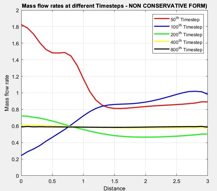
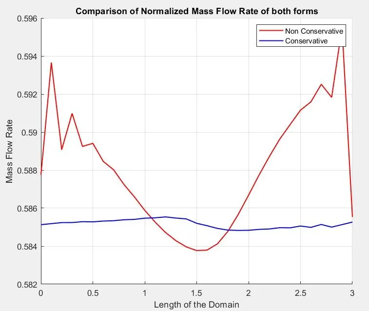
- For the mass flow distribution, conservation form provide better results than the non-conservation form.
- The non-conservation form produce slightly more accurate results for primitive variables. Whereas, the conservation form produces more accurate result for flux terms. So both the forms stand unique on their own in this case.
- In terms of computational effort, conservative form consumes more time. This due to the need to decode the primitive variables from the flux variables. In contrast, non-conservative form requires no such decoding hence consumes less time relative to conservative form.