Week 3.5 - Deriving 4th order approximation of a 2nd order derivative using Taylor Table method
Deriving 4th order approximation of a 2nd order derivative using Taylor Table method
Objectives:
- To derive 4th order approximations (Central Difference Scheme, Skewed Right-sided scheme and Skewed Left-sided scheme) of a second order derivative and prove that our skewed schemes are fourth-order accurate.
- To write program in MATLAB to evaluate the second-order derivative of the analytical function `e^x*cosx` and compare it with the 3 numerical approximations that we have derived.
Derivation of the 4th order approximation of the 2nd order derivative
Central Difference Scheme
Number of Nodes (N) = Number of order of Derivatives (P) + Number of order of approximtions (Q) - 1
Where,
Number of order of Derivatives (P) = 2
Number of order of approximtions (Q) = 4
Therefore,
Number of Nodes (N) = 2 + 4 - 1 => 5
The numerical stencil for the central difference scheme
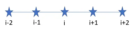
The hypothesis equation for our Central Difference Scheme's Numerical Stencil is
`(∂ ^2 u) /(∂ x^ 2) = a f ( i − 2 ) + b f ( i − 1 ) + c f ( i ) + d f ( i + 1 ) + e f ( i + 2 )` ---------> (1)
where a, b, c, d, and e are coefficients.
The values of coefficients are determined from Taylor Table. In order to create Taylor Table, we need to write the Taylor series expansion for each nodes.
Taylor Series Expansion:
- `a f ( i − 2 ) = ( a ) f ( i ) − ( a ) f ′ ( i ) ( 2 Δ x ) /(1 !) + ( a ) f ′ ' ( i ) ( 2 Δ x ) ^2/ (2 !) − ( a ) f ′ ' ' ( i ) ( 2 Δ x ) ^3 /(3 !) + ( a ) f ′ ' ' ' ( i ) ( 2 Δ x ) ^4 /(4 !) − ( a ) f ′ ' ' ' '( i ) ( 2 Δ x ) ^5 /(5 !) + ( a ) f ′ ' ' ' ' ' ( i ) ( 2 Δ x ) ^6 /(6 !)`
- `b f ( i − 1 ) = ( b ) f ( i ) − ( b ) f ′ ( i ) ( Δ x ) /(1 !) + ( b ) f ′ ' ( i ) ( Δ x ) ^2/ (2 !) − (b) f ′ ' ' ( i ) ( Δ x ) ^3 /(3 !) + ( b ) f ′ ' ' ' ( i ) ( Δ x ) ^4 /(4 !) − ( b ) f ′ ' ' ' '( i ) ( Δ x ) ^5 /(5 !) + ( b ) f ′ ' ' ' ' ' ( i ) ( Δ x ) ^6 /(6 !)`
- `cf(i) = cf(i)`
- `d f ( i + 1 ) = ( d ) f ( i ) + ( d ) f ′ ( i ) ( Δ x ) /(1 !) + ( d ) f ′ ' ( i ) ( Δ x ) ^2/ (2 !) + (d) f ′ ' ' ( i ) ( Δ x ) ^3 /(3 !) + ( d ) f ′ ' ' ' ( i ) ( Δ x ) ^4 /(4 !) + ( d ) f ′ ' ' ' '( i ) ( Δ x ) ^5 /(5 !) + ( d ) f ′ ' ' ' ' ' ( i ) ( Δ x ) ^6 /(6 !)`
- `e f ( i + 2 ) = ( e ) f ( i ) + ( e ) f ′ ( i ) ( 2Δ x ) /(1 !) + ( e ) f ′ ' ( i ) ( 2Δ x ) ^2/ (2 !) + (e) f ′ ' ' ( i ) ( 2Δ x ) ^3 /(3 !) + ( e ) f ′ ' ' ' ( i ) ( 2Δ x ) ^4 /(4 !) + ( e ) f ′ ' ' ' '( i ) ( 2Δ x ) ^5 /(5 !) + ( e ) f ′ ' ' ' ' ' ( i ) ( 2Δ x ) ^6 /(6 !)`
Taylor Table:
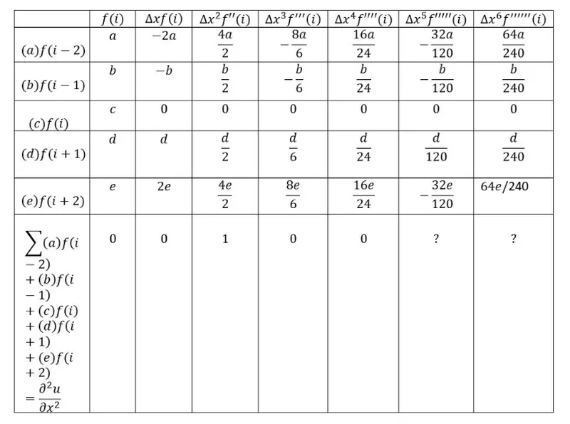
We have five unknowns (a, b, c, d, e) hence we are taking only first five equations as follows:
`a + b + c + d +e=0`
`− 2 a − b + 0 + d + 2 e = 0`
`2 a + b/2 + 0 + d/2 + 2 e = 1`
`− 8 a /6 − b/ 6 + 0 + d /6 + 8 e/ 6 = 0`
`16 a/ 24 + b/ 24 + 0 + d/ 24 + 16 e /24 = 0`
Writing the above equations in Matrix form to determine the values of coefficients (a, b, c, d, e).
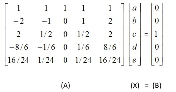
X = inv(A)*B gives the solutions to unknowns.
The values of coefficients are as follows:
`a = − 0.083333`
`b = 1.333333`
`c = − 2.500000`
`d = 1.333333`
`e = − 0.083333`
Proof for fourth order accurate - Central Difference Scheme:
From Taylor table,
`(∂ ^2 u) /( ∂ x^ 2 ) = ( a + b + c + d + e ) f ( i ) + ( − 2 a − b + 0 + d + 2 e ) f ′ ( i ) Δ x + ( 2 a + b/2 + 0 + d/2 + 2 e ) f ′ ' ( i ) Δ x ^2 + ( − 8 /6 a − 1 /6 b + 0 + 1/ 6 d + 8 /6 e ) f ′ ' ' ( i ) Δ x ^3 + ( 16 /24 a + 1 /24 b + 0 + 1 /24 d + 16 /24 e ) f ′ ' ' ' ( i ) Δ x ^4 + ( − 32 /120 a − 1 /120 b + 0 + 1 /120 d + 32 /120 e ) f ′ ' ' ' ' ( i ) Δ x ^5 + ( 64 /240 a + 1 /240 b + 0 + 1/ 240 d + 64 /240 e ) f ′ ' ' ' ' ' ( i ) Δ x ^6`
According to Taylor Table, we are removing the terms which are equals to zero. But the summation of sixth and seventh term of the Taylor's series expansion are undetermined. Hence we consider those as non-zero elements and taken into the equation.
On dividing the above equation's RHS by `(Delta x)^2`, we get:
`(∂ ^2 u) /( ∂ x^ 2 ) = ( 2 a + b/2 + 0 + d/2 + 2 e ) f ′ ' ( i ) + ( − 32 /120 a − 1 /120 b + 0 + 1 /120 d + 32 /120 e ) f ′ ' ' ' ' ( i ) Δ x ^3 +( 64 /240 a + 1 /240 b + 0 + 1/ 240 d + 64 /240 e ) f ′ ' ' ' ' ' ( i ) Δ x ^4`
In the above equation, the term `Δx^4` denotes the truncation error. Here, we can see that the order of the truncation error; [O(`Δx^4`)] is ‘4’. Since we know that the order of approximation is defined by the truncation error term. Therefore, we can say that our central difference scheme is 4th order accurate.
Skewed Right-sided Scheme
Number of Nodes (N) = Number of order of Derivatives (P) + Number of order of approximtions (Q)
Where,
Number of order of Derivatives (P) = 2
Number of order of approximtions (Q) = 4
Therefore,
Number of Nodes (N) = 2 + 4 => 6
The numerical stencil for the Skewed Right-sided scheme
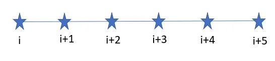
The hypothesis equation for our Skewed Right-sided Scheme's Numerical Stencil is
`(∂ ^2 u) /(∂ x^ 2) = a f ( i ) + b f ( i + 1 ) + c f ( i +2 ) + d f ( i + 3 ) + e f ( i + 4 ) + gf( i + 5 )`---------> (2)
where a, b, c, d, e and g are coefficients.
The values of coefficients are determined from Taylor Table. In order to create Taylor Table, we need to write the Taylor series expansion for each nodes.
Taylor Series Expansion:
- `a f ( i ) = ( a ) f ( i )`
- `b f ( i + 1 ) = ( b ) f ( i ) + ( b ) f ′ ( i ) ( Δ x ) /(1 !) + ( b ) f ′ ' ( i ) ( Δ x ) ^2/ (2 !) + (b) f ′ ' ' ( i ) ( Δ x ) ^3 /(3 !) + ( b ) f ′ ' ' ' ( i ) ( Δ x ) ^4 /(4 !) + ( b ) f ′ ' ' ' '( i ) ( Δ x ) ^5 /(5 !) + ( b ) f ′ ' ' ' ' ' ( i ) ( Δ x ) ^6 /(6 !)`
- `c f ( i + 2 ) = ( c ) f ( i ) + ( c ) f ′ ( i ) ( 2Δ x ) /(1 !) + ( c ) f ′ ' ( i ) ( 2Δ x ) ^2/ (2 !) + (c) f ′ ' ' ( i ) ( 2Δ x ) ^3 /(3 !) + ( c ) f ′ ' ' ' ( i ) ( 2Δ x ) ^4 /(4 !) + ( c ) f ′ ' ' ' '( i ) ( 2Δ x ) ^5 /(5 !) + ( c ) f ′ ' ' ' ' ' ( i ) ( 2Δ x ) ^6 /(6 !)`
- `d f ( i + 3 ) = ( d ) f ( i ) + ( d ) f ′ ( i ) ( 3Δ x ) /(1 !) + ( d ) f ′ ' ( i ) ( 3Δ x ) ^2/ (2 !) + (d) f ′ ' ' ( i ) ( 3Δ x ) ^3 /(3 !) + ( d ) f ′ ' ' ' ( i ) ( 3Δ x ) ^4 /(4 !) + ( d ) f ′ ' ' ' '( i ) ( 3Δ x ) ^5 /(5 !) + ( d ) f ′ ' ' ' ' ' ( i ) ( 3Δ x ) ^6 /(6 !)`
- `e f ( i + 4 ) = ( e ) f ( i ) + ( e ) f ′ ( i ) ( 4Δ x ) /(1 !) + ( e ) f ′ ' ( i ) ( 4Δ x ) ^2/ (2 !) + (e) f ′ ' ' ( i ) ( 4Δ x ) ^3 /(3 !) + ( e ) f ′ ' ' ' ( i ) ( 4Δ x ) ^4 /(4 !) + ( e ) f ′ ' ' ' '( i ) ( 4Δ x ) ^5 /(5 !) + ( e ) f ′ ' ' ' ' ' ( i ) ( 4Δ x ) ^6 /(6 !)`
- `g f ( i + 5 ) = ( g ) f ( i ) + ( g ) f ′ ( i ) ( 5Δ x ) /(1 !) + ( g ) f ′ ' ( i ) ( 5Δ x ) ^2/ (2 !) + (g) f ′ ' ' ( i ) ( 5Δ x ) ^3 /(3 !) + ( g ) f ′ ' ' ' ( i ) ( 5Δ x ) ^4 /(4 !) + ( g ) f ′ ' ' ' '( i ) ( 5Δ x ) ^5 /(5 !) + ( g ) f ′ ' ' ' ' ' ( i ) ( 5Δ x ) ^6 /(6 !)`
Taylor Table:
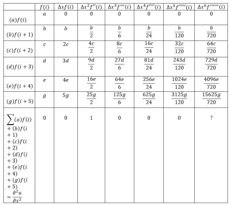
We have six unknowns (a, b, c, d, e, g) hence we are taking only first six equations as follows:
`a + b + c + d + e + g = 0`
`0 + b + 2 c + 3 d + 4 e + 5 g = 0`
`0 + b /2 + 2 c + 9 d/ 2 + 8 e + 25 g/ 2 = 1`
`0 + b /6 + 8 c /6 + 27 d/ 6 + 64 e /6 + 125 g /6 = 0`
`0 + b /24 + 16 c/ 24 + 81 d/ 24 + 256 e/ 24 + 625 g/ 24 = 0`
`0 + b /120 + 32 c /120 + 243 d /120 + 1024 e /120 + 3125 g /120 = 0`
Writing the above equations in Matrix form to determine the values of coefficients (a, b, c, d, e, g).
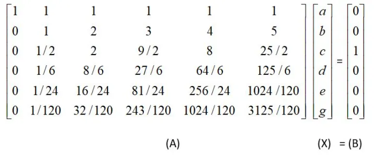
X = inv(A)*B gives the solutions to unknowns.
The values of coefficients are as follows:
`a = 3.75000`
`b = − 12.83333`
`c = 17.83333`
`d = − 13.00000`
`e = 5.08333`
`g = − 0.83333`
Proof for fourth order accurate - Skewed Right-sided Scheme:
From Taylor table,
`(∂ ^2 u) /( ∂ x^ 2 ) = ( a + b + c + d + e + g ) f ( i ) + ( 0 + b + 2 c + 3 d + 4 e + 5 g ) f ′ ( i ) Δ x + ( 0 + b /2 + 4 c /2 + 9 d/ 2 + 16 e /2 + 25 g /2 ) f ′ ' ( i ) Δ x ^2 + ( 0 + b /6 + 8 c /6 + 27 d/ 6 + 64 e/ 6 + 125 g/ 6 ) f ′ ' ' ( i ) Δ x ^3 + ( 0 + b /24 + 16 c /24 + 81 d/ 24 + 256 e /24 + 625 g /24 ) f ′ ' ' ' ( i ) Δ x ^4 + ( 0 + b /120 + 32 c /120 + 243 d /120 + 1024 e /120 + 3125 g/ 120 ) f ′ ' ' ' ' ( i ) Δ x ^5 + ( 0 + b /720 + 64 c/ 720 + 729 d /720 + 4096 e/ 720 + 15625 g /720 ) f ′ ' ' ' ' ' ( i ) Δ x^6`
According to Taylor Table, we are removing the terms which are equals to zero. But the summation of seventh term of the Taylor's series expansion is undetermined. Hence we consider those as non-zero elements and taken into the equation.
On dividing the above equation's RHS by `(Delta x)^2`, we get:
`(∂ ^2 u) /( ∂ x^ 2 ) = ( b/ 2 + 2 c + 9 d /2 + 8 e + 25 g/ 2 ) f ′ ' ( i ) + ( b /720 + 64 c /720 + 729 d/ 720 + 4096 e /720 + 15625 g /720 ) f ′ ' ' ' ' ' ( i ) Δ x^ 4`
In the above equation, the term `Δx^4` denotes the truncation error. Here, we can see that the order of the truncation error; [O(`Δx^4`)] is ‘4’. Since we know that the order of approximation is defined by the truncation error term. Therefore, we can say that our Skewed Right-sided scheme is 4th order accurate.
Skewed Left-sided Scheme
Number of Nodes (N) = Number of order of Derivatives (P) + Number of order of approximtions (Q)
Where,
Number of order of Derivatives (P) = 2
Number of order of approximtions (Q) = 4
Therefore,
Number of Nodes (N) = 2 + 4 => 6
The numerical stencil for the Skewed Left-sided scheme
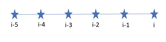
The hypothesis equation for our Skewed Left-sided Scheme's Numerical Stencil is
`(∂ ^2 u) /(∂ x^ 2) = a f ( i-5 ) + b f ( i-4 ) + c f ( i -3 ) + d f ( i -2 ) + e f ( i -1 ) + gf( i )`---------> (3)
where a, b, c, d, e and g are coefficients.
The values of coefficients are determined from Taylor Table. In order to create Taylor Table, we need to write the Taylor series expansion for each nodes.
Taylor Series Expansion:
- `a f ( i - 5 ) = ( a ) f ( i ) - ( a ) f ′ ( i ) ( 5Δ x ) /(1 !) + ( a ) f ′ ' ( i ) ( 5Δ x ) ^2/ (2 !) - (a) f ′ ' ' ( i ) ( 5Δ x ) ^3 /(3 !) + ( a ) f ′ ' ' ' ( i ) ( 5Δ x ) ^4 /(4 !) - ( a ) f ′ ' ' ' '( i ) ( 5Δ x ) ^5 /(5 !) + ( a ) f ′ ' ' ' ' ' ( i ) ( 5Δ x ) ^6 /(6 !)`
- `b f ( i -4) = ( b ) f ( i ) - ( b ) f ′ ( i ) ( 4Δ x ) /(1 !) + ( b ) f ′ ' ( i ) ( 4Δ x ) ^2/ (2 !) - (b) f ′ ' ' ( i ) ( 4Δ x ) ^3 /(3 !) + ( b ) f ′ ' ' ' ( i ) ( 4Δ x ) ^4 /(4 !) - ( b ) f ′ ' ' ' '( i ) ( 4Δ x ) ^5 /(5 !) + ( b ) f ′ ' ' ' ' ' ( i ) ( 4Δ x ) ^6 /(6 !)`
- `c f ( i -3 ) = ( c ) f ( i ) - ( c ) f ′ ( i ) ( 3Δ x ) /(1 !) + ( c ) f ′ ' ( i ) ( 3Δ x ) ^2/ (2 !) - (c) f ′ ' ' ( i ) ( 3Δ x ) ^3 /(3 !) + ( c ) f ′ ' ' ' ( i ) ( 3Δ x ) ^4 /(4 !) - ( c ) f ′ ' ' ' '( i ) ( 3Δ x ) ^5 /(5 !) + ( c ) f ′ ' ' ' ' ' ( i ) ( 3Δ x ) ^6 /(6 !)`
- `d f ( i -2 ) = ( d ) f ( i ) - ( d ) f ′ ( i ) ( 2Δ x ) /(1 !) + ( d ) f ′ ' ( i ) ( 2Δ x ) ^2/ (2 !) - (d) f ′ ' ' ( i ) ( 2Δ x ) ^3 /(3 !) + ( d ) f ′ ' ' ' ( i ) ( 2Δ x ) ^4 /(4 !) - ( d ) f ′ ' ' ' '( i ) ( 2Δ x ) ^5 /(5 !) + ( d ) f ′ ' ' ' ' ' ( i ) ( 2Δ x ) ^6 /(6 !)`
- `e f ( i -1 ) = ( e ) f ( i ) - ( e ) f ′ ( i ) ( Δ x ) /(1 !) + ( e ) f ′ ' ( i ) ( Δ x ) ^2/ (2 !) - (e) f ′ ' ' ( i ) ( Δ x ) ^3 /(3 !) + ( e ) f ′ ' ' ' ( i ) ( Δ x ) ^4 /(4 !) - ( e ) f ′ ' ' ' '( i ) ( Δ x ) ^5 /(5 !) + ( e ) f ′ ' ' ' ' ' ( i ) ( Δ x ) ^6 /(6 !)`
- `g f ( i ) = ( g ) f ( i )`
Taylor Table:
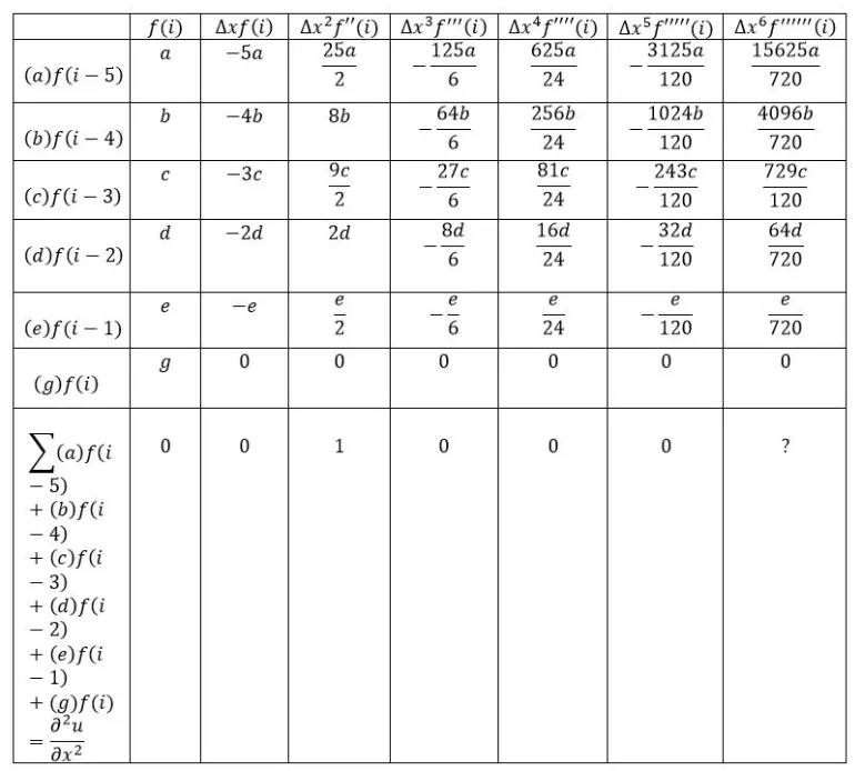
We have six unknowns (a, b, c, d, e, g) hence we are taking only first six equations as follows:
`a + b + c + d + e + g = 0`
`− 5 a − 4 b − 3 c − 2 d − e + 0 = 0`
`25 a/ 2 + 8 b + 9 c/ 2 + 2 d + e /2 + 0 = 1`
`-125 a /6 -64b/6- 27 c /6 -8d/6 -e/6 + 0 = 0`
`625 a /24 + 256 b/ 24 + 81 c /24 + 16 d/24 + e /24 + 0 = 0`
`− 3125 a /120 − 1024 b/ 120 − 243 c/ 120 − 32 d/ 120 − e /120 + 0 = 0`
Writing the above equations in Matrix form to determine the values of coefficients (a, b, c, d, e, g).
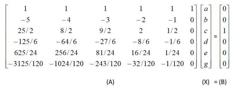
X = inv(A)*B gives the solutions to unknowns.
The values of coefficients are as follows:
`a = − 0.83333`
`b = 5.08333`
`c = − 13.00000`
`d = 17.83333`
`e = − 12.83333`
`g = 3.75000`
Proof for fourth order accurate - Skewed Left-sided Scheme:
From Taylor table,
`(∂ ^2 u) /( ∂ x^ 2 ) = ( a + b + c + d + e + g ) f ( i ) + ( − 5 a − 4 b − 3 c − 2 d − e + 0 ) f ′ ( i ) Δ x + ( 25 a/ 2 + 8 b + 9 c/ 2 + 2 d + e /2 + 0 ) f ′ ' ( i ) Δ x ^2 +( − 125 a/ 6 − 64 b/ 6 − 27 c/ 6 − 8 d/ 6 − e/ 6 + 0 ) f ′ ' ' ( i ) Δ x ^3 + ( 625 a/ 24 + 256 b /24 + 81 c/ 24 + 16 d/ 24 + e /24 + 0 ) f ′ ' ' ' ( i ) Δ x ^4 + ( − 3125 a /120 − 1024 b /120 − 243 c /120 − 32 d/ 120 − e /120 + 0 ) f ′ ' ' ' ' ( i ) Δ x ^5 + ( 15625 a /720 + 4096 b/ 720 + 729 c /720 + 64 d /720 + e /720 + 0 ) f ′ ' ' ' ' ' ( i ) Δ x^6`
According to Taylor Table, we are removing the terms which are equals to zero. But the summation of seventh term of the Taylor's series expansion is undetermined. Hence we consider those as non-zero elements and taken into the equation.
On dividing the above equation's RHS by `(Delta x)^2`, we get:
`(∂ ^2 u) /( ∂ x^ 2 ) = ( 25 a /2 + 8 b + 9 c/ 2 + 2 d + e/ 2 ) f ′ ' ( i ) + ( 15625 a /720 + 4096 b/ 720 + 729 c /720 + 64 d /720 + e /720 ) f ′ ' ' ' ' ' ( i ) Δ x^ 4`
In the above equation, the term `Δx^4` denotes the truncation error. Here, we can see that the order of the truncation error; [O(`Δx^4`)] is ‘4’. Since we know that the order of approximation is defined by the truncation error term. Therefore, we can say that our Skewed Left-sided scheme is 4th order accurate.
Writing program in MATLAB to evaluate the second-order derivative of the analytical function `e^x*cosx` and compare it with the 3 numerical approximations that we have derived
Main Program
clear all
close all
clc
% In this program we are going to derive fourth order approximations for a
% second order derivative using the Taylor Table method
% And compare the results obtained from three different Finite Differencing
% Schemes - Central Differencing Scheme, Skewed Right-sided Scheme and Skewed
% Left-sided Scheme

x = pi/3;

% We need to take series of dx values
dx = linspace(pi/4000,pi/4,100);

for i = 1:length(dx)

    % dx is an array contains 100 elements. For each of this elements,
    % Error is caculated. For each iteration, the corresponding function is
    % called
    central_difference_error(i) = central_difference(x,dx(i));
    skewed_right_sided_error(i) = skewed_right_sided(x,dx(i));
    skewed_left_sided_error(i) = skewed_left_sided(x,dx(i));
end

figure(1)

% loglog function is used to view the graph in log levels (say 10^-1, 10^-6 etc.,)
loglog(dx,central_difference_error,'Color','r','LineWidth',2)
hold on
grid on
loglog(dx,skewed_right_sided_error,'Color','b','LineWidth',2)
hold on
loglog(dx,skewed_left_sided_error,'Color','g','LineWidth',2)
xlabel('dx','FontSize',10)
ylabel('Error','FontSize',10)
legend('Central Difference Scheme','Skewed Right-sided Scheme','Skewed Left-sided Scheme')
Function #1 - Central Difference Scheme
function out = central_difference(x,dx)
% This function is to compute the fourth order approximation of a second
% order derivative using Central Differencing Scheme

% Analytical Function f(x) = exp(x)cos(x)
% Analytical second order derivative f''(x) = -2exp(x)sin(x)

analytical_derivative = -2*exp(x)*sin(x);

a = -0.0833;
b = 1.3333;
c = -2.5000;
d = 1.3333;
e = -0.0833;

% Numerical Analysis
% Central Differencing Scheme = [af(i-2) + bf(i-1) + cf(i) + df(i+1) +
% ef(i+2)]/dx^2

central_difference_scheme = (a*exp(x-2*dx)*cos(x-2*dx) + b*exp(x-dx)*cos(x-dx) + c*exp(x)*cos(x) + d*exp(x+dx)*cos(x+dx) + e*exp(x+2*dx)*cos(x+2*dx))/(dx^2);

out = abs(central_difference_scheme - analytical_derivative);

end
Function #2 - Skewed Right-sided Scheme
function out = skewed_right_sided(x,dx)
% This function is to compute the fourth order approximation of a second
% order derivative using Skewed Right-sided Scheme

% Analytical Function f(x) = exp(x)cos(x)
% Analytical second order derivative f''(x) = -2exp(x)sin(x)

analytical_derivative = -2*exp(x)*sin(x);

a = 3.7500;
b = -12.8333;
c = 17.8333;
d = -13.0000;
e = 5.0833;
g = -0.8333;

% Numerical Analysis
% Central Differencing Scheme = [af(i) + bf(i+1) + cf(i+2) + df(i+3) +
% ef(i+4) + gf(i+5)]/dx^2

skewed_right_sided_scheme = (a*exp(x)*cos(x) + b*exp(x+dx)*cos(x+dx) + c*exp(x+2*dx)*cos(x+2*dx) + d*exp(x+3*dx)*cos(x+3*dx) + e*exp(x+4*dx)*cos(x+4*dx) + g*exp(x+5*dx)*cos(x+5*dx))/(dx^2);

out = abs(skewed_right_sided_scheme - analytical_derivative);

end
Function #3 - Skewed Left-sided Scheme
function out = skewed_left_sided(x,dx)
% This function is to compute the fourth order approximation of a second
% order derivative using Skewed Left-sided Scheme

% Analytical Function f(x) = exp(x)cos(x)
% Analytical second order derivative f''(x) = -2exp(x)sin(x)

analytical_derivative = -2*exp(x)*sin(x);

a = -0.83333;
b = 5.08333;
c = -13.0000;
d = 17.83333;
e = -12.83333;
g = 3.75000;

% Numerical Analysis
% Central Differencing Scheme = [af(i-5) + bf(i-4) + cf(i-3) + df(i-2) +
% ef(i-1) + gf(i)]/dx^2

skewed_left_sided_scheme = (a*exp(x-5*dx)*cos(x-5*dx) + b*exp(x-4*dx)*cos(x-4*dx) + c*exp(x-3*dx)*cos(x-3*dx) + d*exp(x-2*dx)*cos(x-2*dx) + e*exp(x-dx)*cos(x-dx) + g*exp(x)*cos(x))/(dx^2);

out = abs(skewed_left_sided_scheme - analytical_derivative);

end
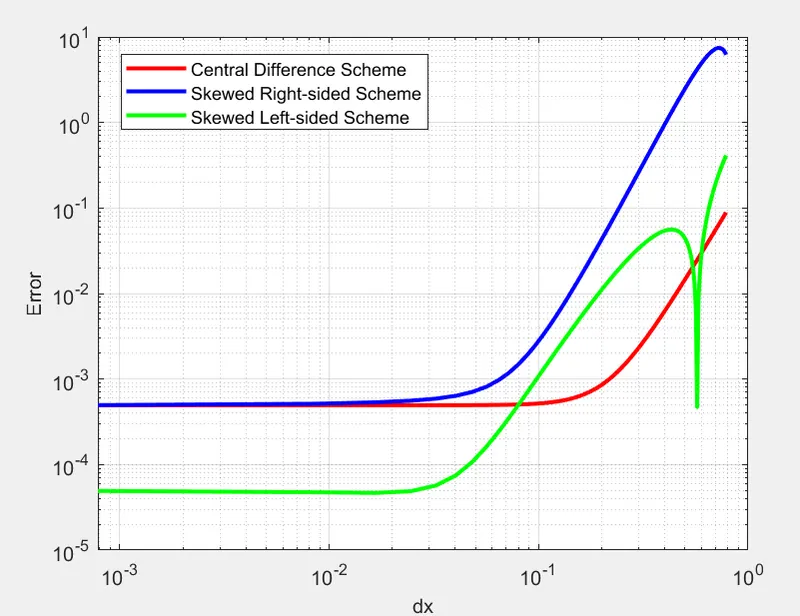
Plot: Dx vs Error
Observation:
From the above plot (Dx vs Error), it is understood that Skewed Left-sided Scheme has least error. Hence, it provides greater accuracy compared to other schemes.
Why a skewed scheme is useful? What can a skewed scheme do that a CD scheme cannot?
Skewed scheme (Right-sided or Left-sided) uses the know values from any one side. Whereas, CD scheme requires data from all the neighbouring sides which are not possible under many circumstances (E.g. boundary or corner nodes).
So Skewed scheme is more beneficial over the CD scheme.