Week 11 - Simulation of Flow through a pipe in OpenFoam
Simulation of Flow through a pipe in OpenFoam
The flow through a pipe is the case of internal flow. The surface is the duct in the case of air; it is a pipe in the case of water. The flow is driven because of the pressure difference created by the pumps, air handling units, fans, etc. They find their major application in the refrigeration and air conditioning industries.
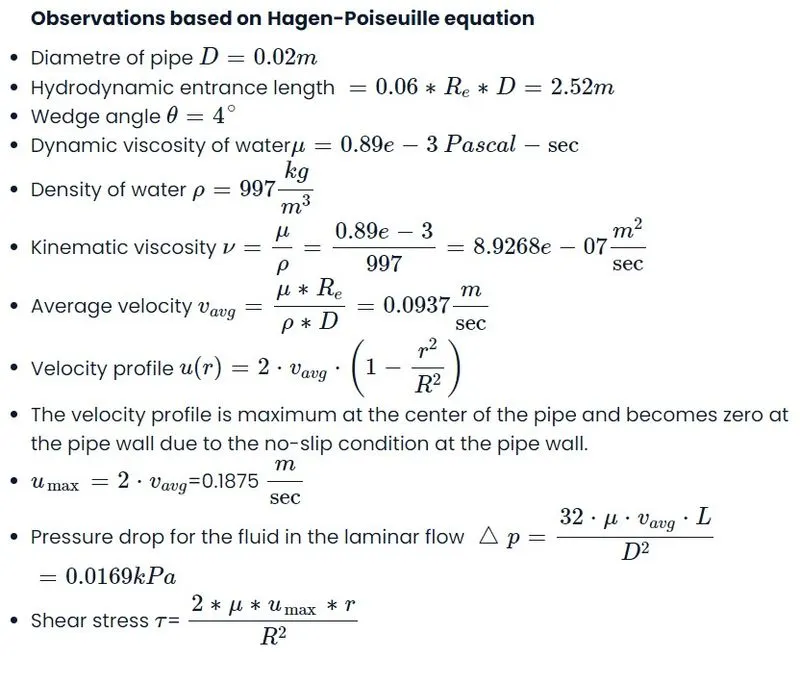
The fluid velocity changes from zero to wall and becomes maximum at the center. In fluid flow, it is preferred to take average velocity because it remains constant when the flow is incompressible, and the cross-sectional area is constant.
Assumptions
- The steady laminar incompressible flow of a fluid is taken.
- There is no velocity in the radial direction.
- There is no acceleration since the flow is steady.
- Reynolds number for the laminar flow is 2100.
- Only the wedge shape of the pipe is considered because the flow is axis-symmetric.
- The equation governing the fluid flow is described by the Hagen-Poiseuille equation.
Objectives of the Project:
(1) Calculation of Flow Variables.
(2) Generation of blockMeshDict using the wedge boundary condition. Create the blockMeshDict file in MATLAB to create the mesh for any wedge angle automatically.
(3) Simulating the pipe flow in OpenFOAM using icoFoam solver.
(4) Post-process the velocity profile and shear stress and compare the simulation results with the Hagen-Poiseuille equation's analytical results.
Hydrodynamic entrance length:
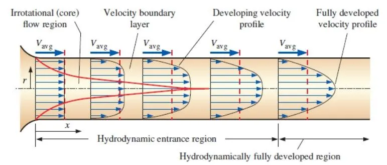
The hydrodynamic entrance region refers to the area of a pipe where fluid entering a pipe develops a velocity profile due to viscous forces spreading from a pipe\'s interior wall. This region has a non-uniform flow. The fluid enters a pipe at a constant speed, so fluid particles in the layer in contact with the pipe\'s surface come to a complete stop because of the no-slip rule. The layer in contact with the pipe surface is resistant to the acceleration of neighboring layers due to viscous forces within the fluid. It slowly slows down adjacent layers of fluid, creating a velocity profile. To keep the mass true, the speed of the fluid layers in the center of the pipe increases to compensate for the reduced speed of the fluid layers near the surface of the pipe. It creates a gradient of velocity across the pipe cross-section.
Matlab Programming:
clear all
close all
clc

% This program is to calculate the following parameters:
% --> Average Velocity (V_avg)
% --> Maximum Velocity (V_max)
% --> Kinematic Pressure (kin_p)
% --> Shear Stress Distribution (tau)

% Wedge angle
theta = 4;

% Reynolds Number [Dimensionless Numebr]
Re  = 2100;

% Density of Water [Kg/m^3]
rho = 997;

% Pipe Diameter [meter]
D = 0.02;

% Dynamic Viscosity of Water @ 25 degrees Celsius [(N.s)/m^2 or Pa.s]
mu = 8.90e-4;

% Kinematic Viscosity
nu = mu/rho;

% Average Velocity [m/s]
V_avg = (Re*mu)/(rho*D);

% Pipe Entry Length: Theoretically, L_h = 0.05*Re*D [m]
L_h = 0.06*Re*D;

% Pipe Total Length: Total Length = Entry Length +
L_tot = L_h+0.3;

% Maximum Velocity
V_max = 2*V_avg;

% Radius of the Pipe
R = D/2;


% Friction factor - Darcy friction factor f
f = 64/Re;

% Pressure Drop/Pressure Loss: It is due to friction of pipe surface [N/m^2]
del_p = (f*L_tot*rho*(V_avg)^2)/(D*2);

% Kinematic Pressure = del_p/rho [m^2 s^-2]
kin_p = del_p/rho;

% Placing some points of radius of the pipe for Shear Stress calculation
r = linspace(-R,R,500);

% The Wall Shear Stress is calculated across the radius of the pipe
for i = 1:length(r)
    tau(i) = (2*mu*V_max*(abs(r(i))))/R^2;
end

plot (tau,r)
xlabel('Shear Stress')
ylabel('Radius')
title('Shear Stress distribution')

header1 = '/*--------------------------------*- C++ -*----------------------------------*\'
header2 = '  =========                 |'
header3 = '  \\      /  F ield         | OpenFOAM: The Open Source CFD Toolbox'
header4 = '   \\    /   O peration     | Website:  https://openfoam.org'
header5 = '    \\  /    A nd           | Version:  10'
header6 = '     \\/     M anipulation  |'
header7 = '\*---------------------------------------------------------------------------*/'
header8 = 'FoamFile'
header9 = '{'
header10 = '    format      ascii;'
header11 = '    class       dictionary;'
header12 = '    object      blockMeshDict;'
header13 = '}'
header14 = '// * * * * * * * * * * * * * * * * * * * * * * * * * * * * * * * * * * * * * //'
header15 = '// ************************************************************************* //'


f1 = fopen('blockMeshDict','w');
fprintf(f1,'%s\n',header1)
fprintf(f1,'%s\n',header2)
fprintf(f1,'%s\n',header3)
fprintf(f1,'%s\n',header4)
fprintf(f1,'%s\n',header5)
fprintf(f1,'%s\n',header6)
fprintf(f1,'%s\n',header7)
fprintf(f1,'%s\n',header8)
fprintf(f1,'%s\n',header9)
fprintf(f1,'%s\n',header10)
fprintf(f1,'%s\n',header11)
fprintf(f1,'%s\n',header12)
fprintf(f1,'%s\n',header13)
fprintf(f1,'%s\n',header14)
fprintf(f1,'convertToMeters 1;')
fprintf(f1,'\n\n')

fprintf(f1,'vertices\n')
fprintf(f1,'(\n')
fprintf(f1,'\t\t (%d %d %d)\n',0,0,0)
fprintf(f1,'\t\t (%d %d %d)\n',0,R*cosd(theta/2),-R*sind(theta/2))
fprintf(f1,'\t\t (%d %d %d)\n',0,R*cosd(theta/2), R*sind(theta/2))
fprintf(f1,'\t\t (%d %d %d)\n',L_tot,0,0)
fprintf(f1,'\t\t (%d %d %d)\n',L_tot,R*cosd(theta/2),-R*sind(theta/2))
fprintf(f1,'\t\t (%d %d %d)\n',L_tot,R*cosd(theta/2), R*sind(theta/2))
fprintf(f1,');\n\n')

fprintf(f1,'blocks\n')
fprintf(f1,'(\n')
fprintf(f1,'\t\t hex (0 3 5 2 0 3 4 1) (%d %d %d) simpleGrading (1 0.1 1)',300,30,1)
fprintf(f1,');\n\n')

fprintf(f1,'edges\n')
fprintf(f1,'(\n')
fprintf(f1,'\t\t arc %d %d (%d %d %d)\n',1,2,0,R,0)
fprintf(f1,'\t\t arc %d %d (%d %d %d)\n',4,5,L_tot,R,0)
fprintf(f1,');\n\n')

fprintf(f1,'boundary\n')
fprintf(f1,'(\n')

fprintf(f1,'\t\t inlet \n')
fprintf(f1, '\t\t { \n')
fprintf(f1,'\t\t\t\t type patch; \n')
fprintf(f1,'\t\t\t\t faces \n')
fprintf(f1,'\t\t\t\t ( \n')
fprintf(f1,'\t\t\t\t\t\t (0 1 2 0) \n')
fprintf(f1,'\t\t\t\t ); \n')
fprintf(f1, '\t\t } \n')

fprintf(f1,'\t\t outlet \n')
fprintf(f1, '\t\t { \n')
fprintf(f1,'\t\t\t\t type patch; \n')
fprintf(f1,'\t\t\t\t faces \n')
fprintf(f1,'\t\t\t\t ( \n')
fprintf(f1,'\t\t\t\t\t\t (3 5 4 3) \n')
fprintf(f1,'\t\t\t\t ); \n')
fprintf(f1, '\t\t } \n')

fprintf(f1,'\t\t top \n')
fprintf(f1, '\t\t { \n')
fprintf(f1,'\t\t\t\t type wall; \n')
fprintf(f1,'\t\t\t\t faces \n')
fprintf(f1,'\t\t\t\t ( \n')
fprintf(f1,'\t\t\t\t\t\t (1 4 5 2) \n')
fprintf(f1,'\t\t\t\t ); \n')
fprintf(f1, '\t\t } \n')

fprintf(f1,'\t\t front \n')
fprintf(f1, '\t\t { \n')
fprintf(f1,'\t\t\t\t type wedge; \n')
fprintf(f1,'\t\t\t\t faces \n')
fprintf(f1,'\t\t\t\t ( \n')
fprintf(f1,'\t\t\t\t\t\t (0 3 4 1) \n')
fprintf(f1,'\t\t\t\t ); \n')
fprintf(f1, '\t\t } \n')

fprintf(f1,'\t\t back \n')
fprintf(f1, '\t\t { \n')
fprintf(f1,'\t\t\t\t type wedge; \n')
fprintf(f1,'\t\t\t\t faces \n')
fprintf(f1,'\t\t\t\t ( \n')
fprintf(f1,'\t\t\t\t\t\t (0 2 5 3) \n')
fprintf(f1,'\t\t\t\t ); \n')
fprintf(f1, '\t\t } \n')

fprintf(f1,'\t\t axis \n')
fprintf(f1, '\t\t { \n')
fprintf(f1,'\t\t\t\t type empty; \n')
fprintf(f1,'\t\t\t\t faces \n')
fprintf(f1,'\t\t\t\t ( \n')
fprintf(f1,'\t\t\t\t\t\t (0 3 3 0) \n')
fprintf(f1,'\t\t\t\t ); \n')
fprintf(f1, '\t\t } \n')

fprintf(f1,');\n\n')

fprintf(f1,'mergePatchPairs\n')
fprintf(f1,'(\n')
fprintf(f1,');\n\n')
fprintf(f1,'%s',header15)
BlockMesh Dict file:
/*--------------------------------*- C++ -*----------------------------------*\
  =========                 |
  \\      /  F ield         | OpenFOAM: The Open Source CFD Toolbox
   \\    /   O peration     | Website:  https://openfoam.org
    \\  /    A nd           | Version:  10
     \\/     M anipulation  |
\*---------------------------------------------------------------------------*/
FoamFile
{
    format      ascii;
    class       dictionary;
    object      blockMeshDict;
}
// * * * * * * * * * * * * * * * * * * * * * * * * * * * * * * * * * * * * * //
convertToMeters 1;

vertices
(
		 (0 0 0)
		 (0 9.993908e-03 -3.489950e-04)
		 (0 9.993908e-03 3.489950e-04)
		 (2.820000e+00 0 0)
		 (2.820000e+00 9.993908e-03 -3.489950e-04)
		 (2.820000e+00 9.993908e-03 3.489950e-04)
);

blocks
(
		 hex (0 1 2 0 3 4 5 3) (50 1 200) simpleGrading (0.4 1 1));

edges
(
		 arc 1 2 (0 1.000000e-02 0)
		 arc 4 5 (2.820000e+00 1.000000e-02 0)
);

boundary
(
		 inlet
		 {
				 type patch;
				 faces
				 (
						 (0 1 2 0)
				 );
		 }
		 outlet
		 {
				 type patch;
				 faces
				 (
						 (3 5 4 3)
				 );
		 }
		 top
		 {
				 type wall;
				 faces
				 (
						 (1 4 5 2)
				 );
		 }
		 front
		 {
				 type wedge;
				 faces
				 (
						 (0 3 4 1)
				 );
		 }
		 back
		 {
				 type wedge;
				 faces
				 (
						 (0 2 5 3)
				 );
		 }
		 axis
		 {
				 type empty;
				 faces
				 (
						 (0 3 3 0)
				 );
		 }
);

mergePatchPairs
(
);

// ************************************************************************* //
Physical Properties file:
/*--------------------------------*- C++ -*----------------------------------*\
  =========                 |
  \\      /  F ield         | OpenFOAM: The Open Source CFD Toolbox
   \\    /   O peration     | Website:  https://openfoam.org
    \\  /    A nd           | Version:  10
     \\/     M anipulation  |
\*---------------------------------------------------------------------------*/
FoamFile
{
    format      ascii;
    class       dictionary;
    location    "constant";
    object      physicalProperties;
}
// * * * * * * * * * * * * * * * * * * * * * * * * * * * * * * * * * * * * * //

nu              [0 2 -1 0 0 0 0] 8.9268e-07;


// ************************************************************************* //
Control Dict file:
/*--------------------------------*- C++ -*----------------------------------*\
  =========                 |
  \\      /  F ield         | OpenFOAM: The Open Source CFD Toolbox
   \\    /   O peration     | Website:  https://openfoam.org
    \\  /    A nd           | Version:  10
     \\/     M anipulation  |
\*---------------------------------------------------------------------------*/
FoamFile
{
    format      ascii;
    class       dictionary;
    location    "system";
    object      controlDict;
}
// * * * * * * * * * * * * * * * * * * * * * * * * * * * * * * * * * * * * * //

application     icoFoam;

startFrom       startTime;

startTime       0;

stopAt          endTime;

endTime         40;

deltaT          0.01;

writeControl    timeStep;

writeInterval   10;

purgeWrite      0;

writeFormat     ascii;

writePrecision  6;

writeCompression off;

timeFormat      general;

timePrecision   6;

runTimeModifiable true;


// ************************************************************************* //
Velocity:
/*--------------------------------*- C++ -*----------------------------------*\
  =========                 |
  \\      /  F ield         | OpenFOAM: The Open Source CFD Toolbox
   \\    /   O peration     | Website:  https://openfoam.org
    \\  /    A nd           | Version:  10
     \\/     M anipulation  |
\*---------------------------------------------------------------------------*/
FoamFile
{
    format      ascii;
    class       volVectorField;
    object      U;
}
// * * * * * * * * * * * * * * * * * * * * * * * * * * * * * * * * * * * * * //

dimensions      [0 1 -1 0 0 0 0];

internalField   uniform (0.0937 0 0);

boundaryField
{

    inlet
    {
        type            fixedValue;
        value           uniform (0.0937 0 0);
    }

    outlet
    {
        type            zeroGradient;

    }

    top
    {
        type            fixedValue;
        value           uniform (0 0 0);
    }
    front
    {
        type            wedge;
    }
    back
    {
        type            wedge;
    }
    axis
    {
        type            empty;
    }


}

// ************************************************************************* //
Pressure:
/*--------------------------------*- C++ -*----------------------------------*\
  =========                 |
  \\      /  F ield         | OpenFOAM: The Open Source CFD Toolbox
   \\    /   O peration     | Website:  https://openfoam.org
    \\  /    A nd           | Version:  10
     \\/     M anipulation  |
\*---------------------------------------------------------------------------*/
FoamFile
{
    format      ascii;
    class       volScalarField;
    object      p;
}
// * * * * * * * * * * * * * * * * * * * * * * * * * * * * * * * * * * * * * //

dimensions      [0 2 -2 0 0 0 0];

internalField   uniform 0;

boundaryField
{
    inlet
    {
        type            zeroGradient;
    }

    outlet
    {
        type            fixedValue;
        value           uniform 0.0189;
    }

    top
    {
        type           zeroGradient;
    }
    front
    {
        type            wedge;
    }
    back
    {
        type            wedge;
    }
    axis
    {
        type            empty;
    }
}

// ************************************************************************* //
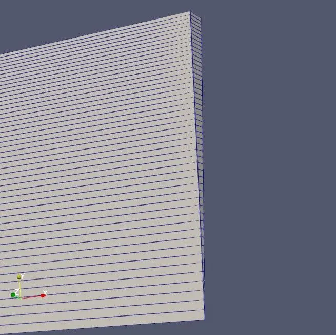
Generated Mesh:
Velocity Profile:
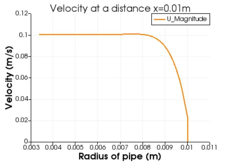
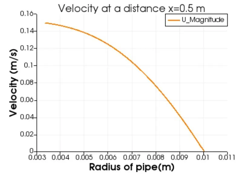
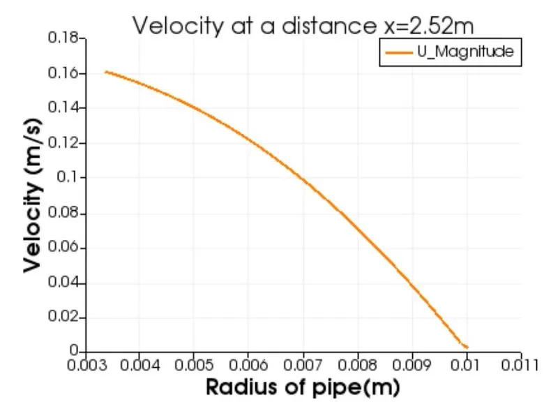
Velocity Plots:
Shear Stress Distribution:
Comparison table:

Conclusion:
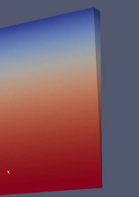
- The velocity profile is plotted at varying distances from the inlet of the pipe.
- The velocity at a distance x = 0.01 from the inlet seems to be slow and stable around the center of the pipe, which shows that the velocity is gradually developing. It suddenly becomes zero at the wall because of the no-slip condition.
- The velocity profile at a distance of x=0.5 and 2.52 is parabolic because the velocity profile moves to the hydrodynamically fully developed region.
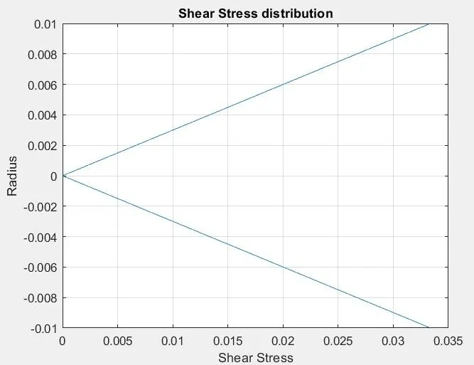
- The shear stress plot is plotted as shown above.
- The irregularities can be observed in the shear stress profile because of the "finite volume method." At node intersections, the value of shear stress increases; this can be reduced by increasing the number of grid points and the computational time.
- The above table shows that the velocity profile calculated numerically equals the Hagen-Poiseuille equation with an error of 0.0275.