Week 5.1 - Mid term project - Solving the steady and unsteady 2D heat conduction problem
Solving the Steady and Unsteady 2D Heat Conduction Problem Using MATLAB
Objective:
To solve the Steady and Unsteady 2D Heat Conduction problem using the point iterative techniques such as Jacobi, Gauss-Seidal and Successive Over Relaxation methods using MATLAB.
Table of Contents
- Objective
- Overview of the Problem
- Steady State 2D Heat Conduction problem
- Discretization
- Implicit Schemes
- MATLAB program to solve the Steady State 2D Heat Conduction problem (Using IMPLICIT Scheme)
- Transient 2D Heat Conduction problem
- Discretization
- Implicit Schemes
- MATLAB program to solve the Transient 2D Heat Conduction problem (Using IMPLICIT Scheme)
- Explicit Scheme
- MATLAB program to solve the Transient 2D Heat Conduction problem (Using EXPLICIT Scheme)
- Comparison of Iterative techniques for both Steady and Unsteady 2D Heat Conduction
- Conclusion
Overview of the Problem
Heat Equation governs the temperature distribution in an object. In our case, we consider an object (i.e, 2D domain) that has length and width as 1 unit.
The Boundary conditions for the problem:
Top Boundary = 600 K
Bottom Boundary = 900 K
Left Boundary = 400 K
Right Boundary = 800 K
The problem is analysed under two conditions:
- Steady State - No change in Temperature with respect to time
- Transient/Unsteady State - Change in Temperature with respect to time
and two Numerical Solution schemes:
- Explicit Scheme - Computation of the dependent variables in terms of known quantities
- Implicit Scheme - Computation of the dependent variables in terms of unknown quantities. Either a matrix or iterative technique is needed to obtin a solution. The iterative techniques for solving implicit equations are:
- Jacobi Method
- Gauss-Seidal Method
- Successive Over Relaxation Method
Steady State 2D Heat Conduction problem
The Steady State 2D Heat Conduction equation is given as follows
`(del^2T)/(delx^2) + (del^2T)/(dely^2) = 0`
Discretization
The above equation is an Elliptical PDE. So discretizing using the Central Difference Scheme which is given by,
`(T_(i-1,j) - 2T_(i,j) + T_(i+1,j))/(Deltax^2) + (T_(i,j-1) - 2T_(i,j) + T_(i,j+1))/(Deltay^2) = 0`
Simplifying we get,
`T_(i,j) = 1/(2(Deltax^2 + Deltay^2)) * ((T_(i-1,j)+T_(i+1,j))/(Deltay^2) + (T_(i,j-1)+T_(i,j+1))/(Deltax^2) )` -------> (A)
Implicit Schemes
Imparting Implicit Schemes to the equation (A) we get,
Jacobi Method
`T_(i,j)^(n+1) = (Deltax^2*Deltay^2)/(2(Deltax^2 + Deltay^2)) * ((T_(i-1,j)+T_(i+1,j))/(Deltax^2) + (T_(i,j-1)+T_(i,j+1))/(Deltay^2))^n`
Gauss-Seidel Method
`T_(i,j)^(n+1) = (Deltax^2*Deltay^2)/(2(Deltax^2 + Deltay^2)) * ((T_(i-1,j)+T_(i+1,j))/(Deltax^2) + (T_(i,j-1)+T_(i,j+1))/(Deltay^2) )^(n+1)`
Successive Over Relaxation Method
`T_(i,j)^(n+1) = (1-omega)*T_(i,j)^(n) + omega * [(Deltax^2*Deltay^2)/(2(Deltax^2 + Deltay^2)) * ((T_(i-1,j)+T_(i+1,j))/(Deltax^2) + (T_(i,j-1)+T_(i,j+1))/(Deltay^2) )^(n+1)]`
where `omega` is the over relaxation factor. Value must be 1.1 or 1.2
MATLAB program to solve the Steady State 2D Heat Conduction problem (Using IMPLICIT Scheme)
Code Overview
For the Steady State 2D Heat Conduction problem, we write a code using Implicit schemes.
Implicit schemes - Jacobi, GS and SOR
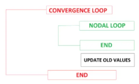
The Steady State 2D Heat Conduction code contains the following algorithm:
Main Program:
clear all
close all
clc

% INPUTS
% Number of nodes along x-axis
nx = 10;

% Number of nodes along y-axis
ny = 10;

x = linspace(0,1,nx);
y = linspace(0,1,ny);

% Grid size in X and y axes
dx = x(2) - x(1);
dy = y(2) - y(1);

% Boundary Conditions
% Defininig the Temperature values at all nodes
T = 300*ones(nx,ny);

% Temperatures (K) on all the sides of the domain
T_T = 600;
T_B = 900;
T_L = 400;
T_R = 800;

T(2:ny - 1, 1)  = T_L;
T(2:ny - 1, nx) = T_R;
T(1, 2:nx - 1)  = T_T;
T(ny, 2:nx - 1) = T_B;

%Calculating Average temperature at corners
T(1,1) = (T_T + T_L)/2;
T(nx,ny) = (T_R + T_B)/2;
T(1,ny) = (T_T + T_R)/2;
T(nx,1) = (T_L + T_B)/2;

% Error and Tolerance criteria
% Taking random error value
error = 9e9;

% Tolerance to converge the solution
tol = 1e-4;
Told = T;
omega = 1.2;

% Iterative Solvers
T_jacobi = ss_jacobi_solver(error,tol,x,y,dx,dy,nx,ny,T,Told);
T_GS = ss_GS_solver(error,tol,x,y,dx,dy,nx,ny,T,Told);
T_SOR = ss_SOR_solver(error,tol,x,y,dx,dy,nx,ny,T,Told,omega);
Function Code for Jacobi Method:
function T = ss_jacobi_solver(error,tol,x,y,dx,dy,nx,ny,T,Told)

jacobi_iter = 1;
% Converge loop
while (error > tol)
    % Space loop
    for i = 2:nx-1
        for j = 2:ny-1
          T(i,j) = (1/(2*(dx^2 + dy^2)))*((Told(i-1,j) + Told(i+1,j))*dy^2 + (Told(i,j-1) + Told(i,j+1))*dx^2);
        end
    end
    error = max(max(abs(Told - T)));
    Told = T;
    jacobi_iter = jacobi_iter + 1;

    %Plotting
    figure(1)
    contourf(x,y,T)
    clabel(contourf(x,y,T))
    colorbar
    colormap(jet)
    set(gca, 'ydir', 'reverse')
    xlabel('X-Axis')
    ylabel('Y-Axis')
    title(sprintf('No. of Jacobi Iterations(IMPLICIT) = %d', jacobi_iter));
end

end
Function Code for Gauss-Seidal Method:
function T = ss_GS_solver(error,tol,x,y,dx,dy,nx,ny,T,Told)

GS_iter = 1;
% Converge loop
while (error > tol)
    % Space loop
    for i = 2:nx-1
        for j = 2:ny-1
          T(i,j) = (1/(2*(dx^2 + dy^2)))*((T(i-1,j) + Told(i+1,j))*dy^2 + (T(i,j-1) + Told(i,j+1))*dx^2);
        end
    end
    error = max(max(abs(Told - T)));
    Told = T;
    GS_iter = GS_iter + 1;

    %Plotting
    figure(2)
    contourf(x,y,T)
    clabel(contourf(x,y,T))
    colorbar
    colormap(jet)
    set(gca, 'ydir', 'reverse')
    xlabel('X-Axis')
    ylabel('Y-Axis')
    title(sprintf('No. of GS Iterations(IMPLICIT) = %d', GS_iter));
end

end
Function Code for Successive Over Relaxation Method:
function T = ss_SOR_solver(error,tol,x,y,dx,dy,nx,ny,T,Told,omega)

SOR_iter = 1;
% Converge loop
while (error > tol)
    % Space loop
    for i = 2:nx-1
        for j = 2:ny-1
          T(i,j) = (omega*(1/(2*(dx^2 + dy^2)))*((T(i-1,j) + Told(i+1,j))*dy^2 + (T(i,j-1) + Told(i,j+1))*dx^2)) + ((1-omega)*Told(i,j));
        end
    end
    error = max(max(abs(Told - T)));
    Told = T;
    SOR_iter = SOR_iter + 1;

    %Plotting
    figure(3)
    contourf(x,y,T)
    clabel(contourf(x,y,T))
    colorbar
    colormap(jet)
    set(gca, 'ydir', 'reverse')
    xlabel('X-Axis')
    ylabel('Y-Axis')
    title(sprintf('No. of SOR Iterations(IMPLICIT) = %d', SOR_iter));
end

end
Outputs
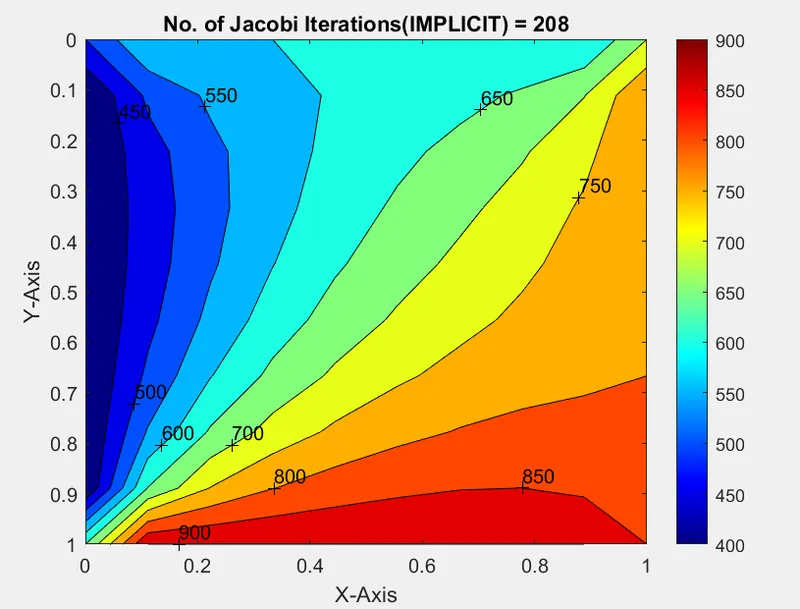
Plot for Jacobi solver:
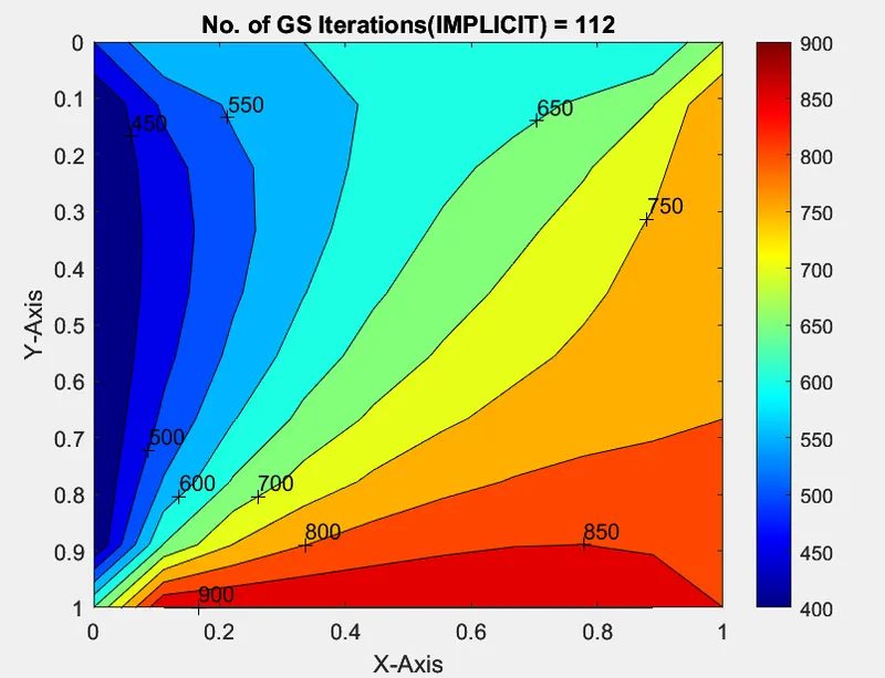
Plot for Gauss Seidal Method
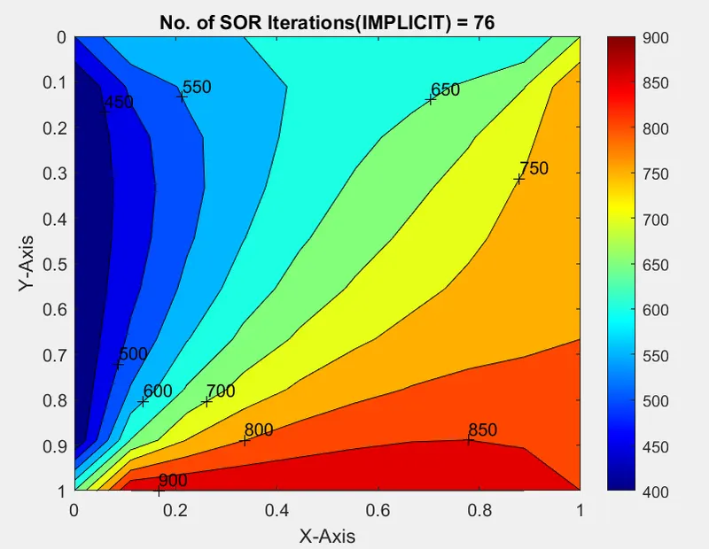
Plot for Successive Over Relaxation Method
Transient 2D Heat Conduction Problem
The Transient 2D Heat Conduction equation is given by,
`(delT)/(delt) - alpha* ((del^2t)/(delx^2) + (del^2t)/(dely^2)) = 0`
`(delT)/(delt) =alpha ((del^2t)/(delx^2) + (del^2t)/(dely^2))` -----------> (2)
where `alpha` is the Thermal Diffusivity (It measures the rate of transfer of heat of a material from the hot end to the cold end).
Discretization
In the above equation (2), LHS side is Hyperbolic PDE and RHS side is Elliptical PDE.
For the Hyperbolic PDE, Forward Difference method is used for discretization.
For the Elliptical PDE, Central Difference method is used for discretization.
Hence the discretized Transient 2D Heat Conduction is given by,
`(T_(i,j)^(n+1) - T_(i,j)^n)/(Deltat) = alpha[(T_(i-1,j)-2T_(i,j)+T_(i+1,j))/(Deltax^2) + (T_(i,j-1)-2T_(i,j)+T_(i,j+1))/(Deltay^2)]^n`
Rearranging we get,
`T_(i,j)^(n+1) = T_(i,j)^n + alphaDeltat[(T_(i-1,j)-2T_(i,j)+T_(i+1,j))/(Deltax^2) + (T_(i,j-1)-2T_(i,j)+T_(i,j+1))/(Deltay^2)]^n`
`T_(i,j)^(n+1) = T_(i,j)^n + k_1[T_(i-1,j)-2T_(i,j)+T_(i+1,j)]^n + k_2[T_(i,j-1)-2T_(i,j)+T_(i,j+1)]^n` -----------> (B)
where,
`k_1 = (alphaDeltat)/(Deltax^2)`
`k_2 = (alphaDeltat)/(Deltay^2)`
Implicit Schemes
Imparting the implicit schemes to the above equation (B) we get,
Jacobi Method
`T_(i,j)^(n+1) = T_(i,j)^n + k_1[T_(i-1,j)-2T_(i,j)+T_(i+1,j)]^n + k_2[T_(i,j-1)-2T_(i,j)+T_(i,j+1)]^n`
Gauss Seidal Method
`T_(i,j)^(n+1) = T_(i,j)^n + k_1[T_(i-1,j)-2T_(i,j)+T_(i+1,j)]^(n+1) + k_2[T_(i,j-1)-2T_(i,j)+T_(i,j+1)]^(n+1)`
Successive Over Relaxation Method
`T_(i,j)^(n+1) = (1-omega)T_(i,j)^n + omega(T_(i,j)^n + k_1[T_(i-1,j)-2T_(i,j)+T_(i+1,j)]^(n+1) + k_2[T_(i,j-1)-2T_(i,j)+T_(i,j+1)]^(n+1))`
where `omega` is the Over relaxation factor and the value must be 1.1 or 1.2.
MATLAB program to solve the Transient 2D Heat Conduction problem (Using IMPLICIT Scheme)
Code Overview
For the Transient 2D Heat Conduction problem, we write a code using Implicit schemes.
Implicit schemes - Jacobi, GS and SOR
The Transient 2D Heat Conduction code contains the following algorithm:
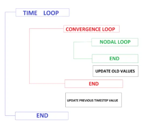
Main Program
clear all
close all
clc

% INPUTS
% Number of nodes along x-axis
nx = 10;

% Number of nodes along y-axis
ny = 10;
nt = 1400; % Time steps

x = linspace(0,1,nx);
y = linspace(0,1,ny);

% Grid size in X and y axes
dx = x(2) - x(1);
dy = y(2) - y(1);
dt = 1e-3;

% Boundary Conditions
% Defininig the Temperature values at all nodes
T = 300*ones(nx,ny);

% Temperatures (K) on all the sides of the domain
T_T = 600;
T_B = 900;
T_L = 400;
T_R = 800;

T(2:ny - 1, 1)  = T_L;
T(2:ny - 1, nx) = T_R;
T(1, 2:nx - 1)  = T_T;
T(ny, 2:nx - 1) = T_B;

%Calculating Average temperature at corners
T(1,1) = (T_T + T_L)/2;
T(nx,ny) = (T_R + T_B)/2;
T(1,ny) = (T_T + T_R)/2;
T(nx,1) = (T_L + T_B)/2;

% Error and Tolerance criteria
% Taking random error value
error = 9e9;

% Tolerance to converge the solution
tol = 1e-4;
Told = T;
Tinit = T;
alpha = 1.4; % Specific heat ratio
omega = 1.1; % Relaxation factor

% Iterative Solvers
T_jacobi = transient_jacobi_solver(tol,x,y,dx,dy,nx,ny,T);
T_GS = transient_GS_solver(tol,x,y,dx,dy,nx,ny,T);
T_SOR = transient_SOR_solver(tol,x,y,dx,dy,nx,ny,T);
Function Code for Jacobi Method
function T = transient_jacobi_solver(tol,x,y,dx,dy,nx,ny,T)
nt = 1400;
dt = 1e-3;
Told = T;
Tinit = T;
alpha = 1.4;
k1 = alpha*(dt/(dx^2));
k2 = alpha*(dt/(dy^2));

jacobi_iter = 1;
% Time loop
for k = 1:nt
    error = 9e9;
% Converge loop
while (error > tol)
    % Space loop
    for i = 2:nx-1
        for j = 2:ny-1

          term1 = Tinit(i,j);
          term2 = k1*(Told(i-1,j)-2*(Tinit(i,j))+Told(i+1,j));
          term3 = k2*(Told(i,j-1)-2*(Tinit(i,j))+Told(i,j+1));
          T(i,j) = term1 + term2 + term3;
        end
    end
    error = max(max(abs(Told - T)));
    Told = T;
    jacobi_iter = jacobi_iter + 1;

end

Tinit = T;
 %Plotting
    figure(4)
    contourf(x,y,T)
    clabel(contourf(x,y,T))
    colorbar
    colormap(jet)
    set(gca, 'ydir', 'reverse')
    xlabel('X-Axis')
    ylabel('Y-Axis')
    title(sprintf('No. of Jacobi Iterations(IMPLICIT) = %d', jacobi_iter));
end

end
Function Code for Gauss Seidal Method
function T = transient_GS_solver(tol,x,y,dx,dy,nx,ny,T)
nt = 1400;
dt = 1e-3;
Told = T;
Tinit = T;
alpha = 1.4;
k1 = alpha*(dt/(dx^2));
k2 = alpha*(dt/(dy^2));

GS_iter = 1;
% Time loop
for k = 1:nt
    error = 9e9;
% Converge loop
while (error > tol)
    % Space loop
    for i = 2:nx-1
        for j = 2:ny-1

          term1 = Tinit(i,j);
          term2 = k1*(T(i-1,j)-2*(Tinit(i,j))+Told(i+1,j));
          term3 = k2*(T(i,j-1)-2*(Tinit(i,j))+Told(i,j+1));
          T(i,j) = term1 + term2 + term3;
        end
    end
    error = max(max(abs(Told - T)));
    Told = T;
    GS_iter = GS_iter + 1;

end

Tinit = T;
 %Plotting
    figure(5)
    contourf(x,y,T)
    clabel(contourf(x,y,T))
    colorbar
    colormap(jet)
    set(gca, 'ydir', 'reverse')
    xlabel('X-Axis')
    ylabel('Y-Axis')
    title(sprintf('No. of GS Iterations(IMPLICIT) = %d', GS_iter));
end

end
Function Code for Successive Over Relaxation Method
function T = transient_SOR_solver(tol,x,y,dx,dy,nx,ny,T)
nt = 1400;
dt = 1e-3;
Told = T;
Tinit = T;
alpha = 1.4;
omega = 1.1;
k1 = alpha*(dt/(dx^2));
k2 = alpha*(dt/(dy^2));

SOR_iter = 1;
% Time loop
for k = 1:nt
    error = 9e9;
% Converge loop
while (error > tol)
    % Space loop
    for i = 2:nx-1
        for j = 2:ny-1

          term1 = Tinit(i,j);
          term2 = k1*(T(i-1,j)-2*(Tinit(i,j))+Told(i+1,j));
          term3 = k2*(T(i,j-1)-2*(Tinit(i,j))+Told(i,j+1));
          T(i,j) = omega*(term1 + term2 + term3)+((1-omega)*Told(i,j));
        end
    end
    error = max(max(abs(Told - T)));
    Told = T;
    SOR_iter = SOR_iter + 1;

end

Tinit = T;
 %Plotting
    figure(6)
    contourf(x,y,T)
    clabel(contourf(x,y,T))
    colorbar
    colormap(jet)
    set(gca, 'ydir', 'reverse')
    xlabel('X-Axis')
    ylabel('Y-Axis')
    title(sprintf('No. of SOR Iterations(IMPLICIT) = %d', SOR_iter));
end

end
Outputs
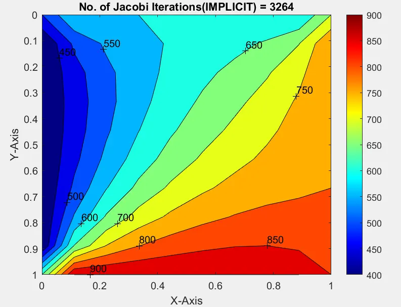
Plot for Jacobi Solver
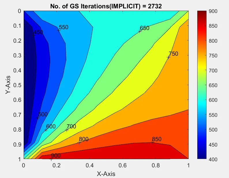
Plot for Gauss Seidal Solver
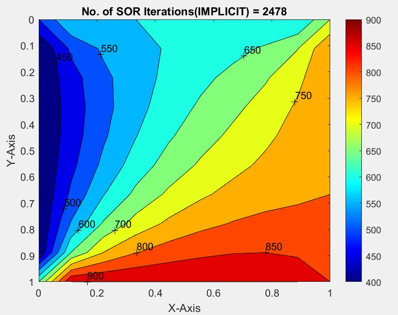
Plot for Successive Over Relaxation Solver
Explicit Scheme
Rewriting the Transient 2D Heat Conduction equation
`(delT)/(delt) =alpha ((del^2t)/(delx^2) + (del^2t)/(dely^2))`
where,
`alpha` is the Thermal Diffusivity.
Discretizing and writing the Explicit scheme for the above equation is given by,
`T_(i,j)^(n+1) = T_(i,j)^n + k_1[T_(i-1,j)-2T_(i,j)+T_(i+1,j)]^n + k_2[T_(i,j-1)-2T_(i,j)+T_(i,j+1)]^n`
where,
`k_1 = (alphaDeltat)/(Deltax^2)`
`k_2 = (alphaDeltat)/(Deltay^2)`
MATLAB program to solve the Transient 2D Heat Conduction problem (Using Explicit Scheme)
Main Program
clear all
close all
clc

% INPUTS
% Number of nodes along x-axis
nx = 10;

% Number of nodes along y-axis
ny = 10;
nt = 1400; % Time steps

x = linspace(0,1,nx);
y = linspace(0,1,ny);

% Grid size in X and y axes
dx = x(2) - x(1);
dy = y(2) - y(1);
dt = 1e-3;

% Boundary Conditions
% Defininig the Temperature values at all nodes
T = 300*ones(nx,ny);

% Temperatures (K) on all the sides of the domain
T_T = 600;
T_B = 900;
T_L = 400;
T_R = 800;

T(2:ny - 1, 1)  = T_L;
T(2:ny - 1, nx) = T_R;
T(1, 2:nx - 1)  = T_T;
T(ny, 2:nx - 1) = T_B;

%Calculating Average temperature at corners
T(1,1) = (T_T + T_L)/2;
T(nx,ny) = (T_R + T_B)/2;
T(1,ny) = (T_T + T_R)/2;
T(nx,1) = (T_L + T_B)/2;

% Error and Tolerance criteria
% Taking random error value
error = 9e9;

% Tolerance to converge the solution
tol = 1e-4;
Told = T;
alpha = 1.4; % Specific heat ratio
k1 = alpha*(dt/(dx^2));
k2 = alpha*(dt/(dy^2));


% Iterative Solvers

transient_explicit_iter = 1;
% Time loop
for k = 1:nt
    error = 9e9;
% Converge loop
while (error > tol)
    % Space loop
    for i = 2:nx-1
        for j = 2:ny-1

          term1 = Told(i,j);
          term2 = k1*(Told(i-1,j)-2*(Told(i,j))+Told(i+1,j));
          term3 = k2*(Told(i,j-1)-2*(Told(i,j))+Told(i,j+1));
          T(i,j) = term1 + term2 + term3;
        end
    end
    error = max(max(abs(Told - T)));
    Told = T;
    transient_explicit_iter = transient_explicit_iter + 1;
    %Plotting
    figure(7)
    contourf(x,y,T)
    clabel(contourf(x,y,T))
    colorbar
    colormap(jet)
    set(gca, 'ydir', 'reverse')
    xlabel('X-Axis')
    ylabel('Y-Axis')
    title(sprintf('No. of Jacobi Iterations(EXPLICIT) = %d', transient_explicit_iter));

end

end
Output
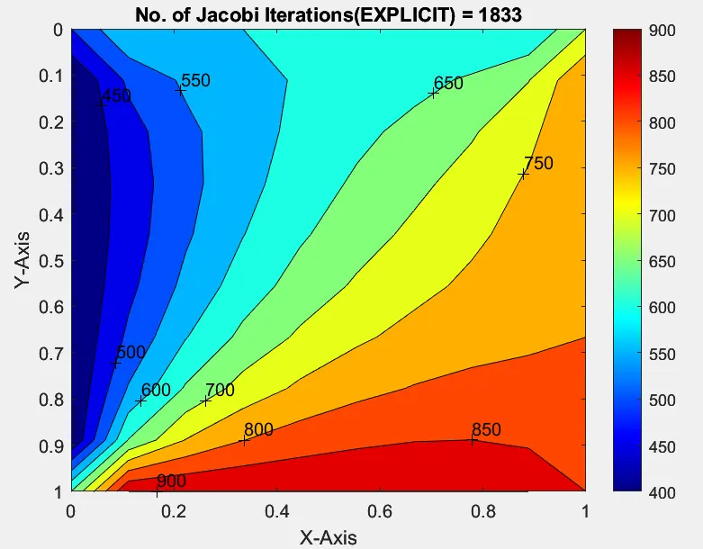
Plot for Explicit scheme
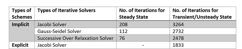
Comparison of Iterative Technique for both Steady and Unsteady 2D Heat Conduction
Conclusions
Hence the steady and unsteady 2D Heat Conduction problem is solved using the point iterative technique in MATLAB.
From the result, it is observed that the Successive Over Relaxation Solver (for both steady and unsteady states) uses less computation effort to reach the solution or solution gets converged with less computational effort.