Week 9 - FVM Literature Review
FVM LITERATURE REVIEW
In computational fluid dynamics, the three classical choices for the numerical solution of PDEs are,
1. Finite difference method (FDM)
2. Finite element method (FEM)
3. Finite volume method (FVM)
finite difference method (FDM):
The FDM is the oldest and is based upon applying a local Taylor expansion to approximate the differential equations. The grid is linear and aligned so that all grid points lie straight. Here, the properties are considered to be concentrated at a single point.
In finite element method (FEM):
The properties are valid over an elemental area. the properties assumed to be concentrated at the area center.
In finite volume method (FVM):
The method is applied over a volume such that the governing equation is valid over the entire volume. The properties are assumed to be concentrated at the geometric center of the control volume.
Finite Volume Method(FVM):
- The Finite volume method(FVM) is a method for representing and evaluating partial differential equations in form of algebraic equations.
- This method integrates volume into a partial differential equation containing a divergence term and is converted into surface integrals, using the divergence theorem. These terms are then evaluated as fluxes at the surfaces of each finite volume. Because the flux entering a given volume is identical to that leaving the adjacent volume, these methods are conservative.
- 'Finite volume' refers to the small volume surrounding each node point on a mesh.
- The advantage of the finite volume method is that it is easily formulated to allow unstructured meshes and this method is used in many computational fluid dynamic packages.
Differences between FDM & FVM:
- A finite difference method(FDM) discretization is based upon the differential form of the PDE to be solved. Each derivative is replaced with an approximate difference formula that can generally be derived from a Taylor series expansion.
- A finite volume method(FVM) discretization is based upon an integral form of PDE to be solved. The computational domain is discretized into finite volumes and then for every volume, the governing equations are solved. The resulting system of the equation usually involves fluxes of the conserved variables, and thus the calculation of fluxes is very important in FVM.
- The FVM is most commonly used in many computational fluid dynamic packages.
- The basic advantage of FVM over FDM is it does not require the use of structured grids, and the effort to convert the given mesh into a structured numerical grid internally is completely avoided.
Gradient Scheme:
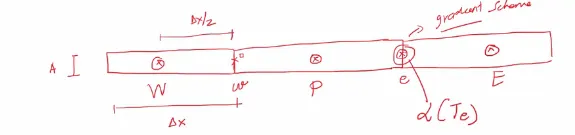
Let us consider the control volumes W, P, and E. When we calculate the temperature gradient in the east face (at e), we basically use temperature from neighboring points trying to evaluate or numerically represent the gradient of temperature (like at P and E). This scheme is called as Gradient scheme.
Interpolation scheme:
The approximation of surface and volume integrals may require values of the variable at locations other than the computational nodes of the Control Volume (CV). Values at these locations are obtained using a certain interpolation scheme. Some of the widely used interpolation schemes are as follow,
1. Upwind Interpolation Scheme (UDS)
2. Linear Interpolation Scheme (CDS)
3. Quadratic Upwind Interpolation Scheme (QUICK)
4. Hybrid Interpolation Scheme
5. Total variation Diminishing Scheme (TVD)
6. Essentially Non-oscillatory interpolation Scheme (ENO).
1) Upwind Interpolation Scheme (UDS):
- In this method, the direction of velocity at the point determines the variable values to be used in the interpolation process.
- Makes use of node that is upwind to the node that is considered.
- The UDS is the only approximation that satisfies the boundness criterion unconditionally.
- Mainly used for convection-dominated problems.
- This interpolation scheme uses a backward or forward finite difference approximation (depending on the flow direction).
- UDS is only first-order accurate, Thus requiring a finer grid for accurate solutions.
- The UDS is very popular for its solution stability.

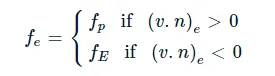
The upwind interpolation (UDS) for approximating the value of a variable at the east face (e) connecting the control volumes P and E is given by,
2) Linear Interpolation Scheme (CDS):
- We can approximate the value of the variable at the CV face center by linear interpolation of the values at the two nearest computational nodes.
- This is equivalent to the use of the central difference scheme of first-order derivative, and hence it is also known as the central difference scheme.
- CDS is second-order accurate.
- This scheme may produce oscillatory solutions.
- It is the simplest and most widely used scheme.
- Used for turbulent flows using large eddy simulations or direct numerical simulation.
Thus, at location 'e' on a Cartesian grid, the variable value is approximated by;

3) Quadratic Upwind Interpolation Scheme (QUICK):
- This approximates the value of a variable at the CV face center by quadratic interpolation of the values at the three nearest computational nodes (one downstream node, D, and two upstream nodes, U).
- Leonard (1979) named this scheme QUICK(Quadratic Upwind Interpolation for Convective Kinematics).
- It has better damping than CDS and better accuracy than UDS.
- For the east face
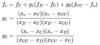
where if the flow is along the positive x-axis,
D will be E
U will be P
UU will be W
- It is third-order accurate for both uniform and nonuniform grids.
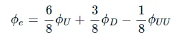
- For a uniform grid, the simplified form is given by,
- This scheme still has problems with oscillation but is not as severe as CDS.
4) Hybrid Interpolation Scheme:
It is the blend of Linear Interpolation Scheme (CDS) and Upwind Interpolation Scheme (UDS) schemes, based on the Peclet number.

5) Total variation Diminishing Scheme (TVD):
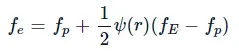
where ψ is the flux limiter.
Flux Limiters:
- For convective fluid flow, it is observed that the low order schemes are usually stable but quite dissipative in nature around the points of discontinuity or shocks while the higher order schemes are unstable in nature and show oscillations in the vicinity of discontinuity or shocks.
- Highly accurate and oscillation-free schemes are known as High-Resolution Schemes.
- Flux limiters are used in the high-resolution schemes which are used to solve the problems in fluid dynamics PDEs.
- They are used in a high-resolution scheme to avoid the spurious oscillation that would otherwise occur with a high-order spatial discretization scheme due to shocks, discontinuities, or sharp changes in the solution domain.
- The use of flux limiters together with an appropriate high-resolution scheme makes the solution stable.
- In, the total variation diminishing (TVD) scheme,

where,
`f^(low)` = Low precision flux (1st order accurate)
`f^(high)` = High precision flux (Highest order accurate)
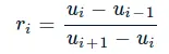
`phi(r)` = flux limiter function and r represent the ratio of successive gradients on solution mesh
REFERENCES: