Simulating a 2nd order ODE system of a simple pendulum

Objective:

To simulate the motion of a simple pendulum by using the given 2nd order ODE and to create the animation of its motion by using a MATLAB code.

Theory:

ODE: Ordinary Differential Equation, is a differential equation containing one or more functions of one independent variable and the derivatives of those functions.

Second-Order ODE: They are ODE with the form ay″+by′+cy=0">ay′′+by′+cy=0ay″+by′+cy=0

The following second-order ODE represents the equation of motion of a simple pendulum with damping,

In the above equation,

g = gravity in (m/s^2)

L = length of the pendulum in (m)

m = mass of the ball in (kg)

b =damping coefficient (no units)

θ =angular displacement

solving the equation,

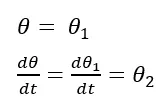
consider above equation as equation 1,

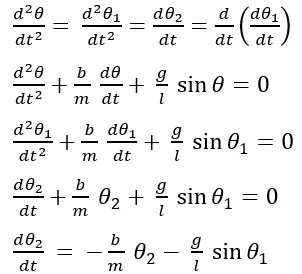
consider above equation as equation 2, thus the 2nd order ODE is broken down into 1st order ODEs (that is equation 1 & 2)

Therefore, the solution set dtheta/dt is given by,

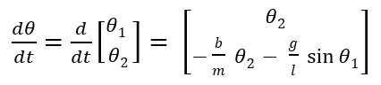
ode45: It is a versatile ODE solver used in MATLAB to solve most of the problems. They are used to solve first order Ordinary Differential Equations

anonymous function: An anonymous function is a function that is not stored in a program file, but is associated with a variable whose data type is function_handle.

Code:

Function code:

function [dtheta_dt]=ode_func(t,theta,b,g,l,m)
theta1=theta(1);
theta2=theta(2);
dtheta1_dt=theta2;
dtheta2_dt=-(b/m)*theta2-(g/l)*sin(theta1);
dtheta_dt=[dtheta1_dt;dtheta2_dt];
end

• the above subprogram is a function code that is later called in the main program to solve the ordinary differential equation.
• the inputs for the function are time(t), displacement(theta), damping coefficient(d), gravity(g), length of pendulum (l) and mass(m).
• the output of this function is the solution set consisting of angular displacement(θ1) and angular velocity(θ2).

Main code:

The MATLAB code is given below,

%simple pendulum velocity for different displacement is calculated
clear all
close all
clc

%Inputs given
%length(L)=1 m,
l=1;
%mass(m)=1 kg,
m=1;
%damping_coefficient(b)=0.05,
b=0.05;
%specific_gravity(g)=9.81 m/s^2
g=9.81;

%initial coditions
%initial angular_displacement and angular_velocity(rad/s)
theta_0=[0;3];
%time_span in (s)
tspan=linspace(0,20,750);

%solve ODE
[t,results]=ode45(@(t,theta)ode_func(t,theta,b,g,l,m),tspan,theta_0);

%ODE plotting
figure(1)
title('Simple pendulum')
plot(t,results(:,1))
hold on
plot(t,results(:,2))
grid on
legend("Displacement","Velocity")
xlabel('Time')
ylabel('Plot')

%animation inputs
x0=0;
y0=0;

%the displacement (theta_1)
t=results(:,1);
frame = 1;

for i=1:length(t)
    theta1=(t(i));
    
    %resolving theta_1 with respect to X and Y axes
    x1=-l*sin(theta1);
    y1=-l*cos(theta1);
    
    %plotting for animation
    figure(2)
    %plotting connecting_rod 
    plot([x0,x1],[y0,y1],'linewidth',2)
    %plotting bob
    viscircles([x1,y1],0.05,'color','r','linewidth',15)
    %plotting fixed_support
    rectangle('position',[-1.5,0,3,0.25],'facecolor','black')
    grid on
    axis([-1.5,1.5,-1.5,1.5])
    pause(0.009)
    mv(frame)=getframe(gcf);
    frame=frame+1;
end

%creating movie
video=VideoWriter('simple_pendulum_challenge.AVI','MPEG-4');
open(video)
writeVideo(video,[mv])
close(video)

• the inputs and initial conditions are assigned in the first part of the program.
• an anonymous function is used to solve the ode45 solver. The inputs are followed by initial conditions in an anonymous function. The LHS of the anonymous function uses a function handle that is used to pass a function to another function.
• the function 'ode_fun' is called here using an anonymous function.
• the outputs of function are time period (t) and results (which is a solution set of angular displacement and angular velocity) which are used for plotting 'time vs displacement' and 'time vs velocity' graphs.
• for animation, the theta 1(displacement) is resolved to x and y axes. -1 is multiplied as the pendulum is facing downwards.
• the plot consists of a fixed beam in which the pendulum is mounted.
• pause command pauses the plot for the specified seconds.
• for each displacement value, a plot is made and stored as a frame for animation in variable 'mv'.
• to create a movie first, a file is created, then the file is opened and the frames in variable 'mv' are written to it, then the file is closed.
• after running successfully, a video file in a specified format is created in the working directory.

Results:

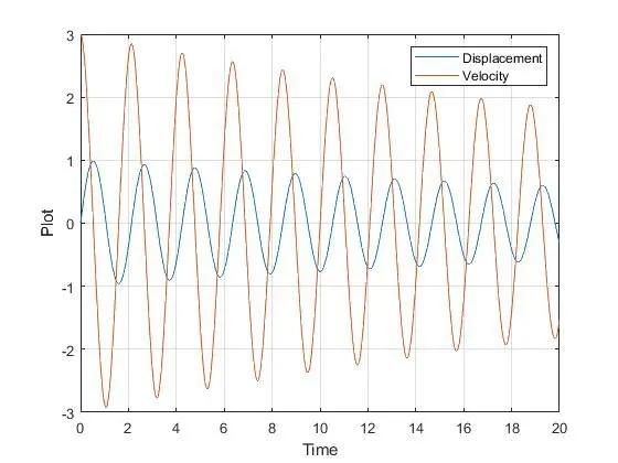
The program for simulating a 2nd order ODE system of a simple pendulum has been coded successfully. The output plot has been obtained and the animation is generated,

1. the plot ' time vs angular displacement and velocity '

2. the animation of the simple pendulum can be viewed on youtube by using the below link,

https://youtu.be/dBYnIED_yWc