Week 3.5 - Deriving 4th order approximation of a 2nd order derivative using Taylor Table method

DERIVING 4TH ORDER APPROXIMATION OF A 2ND ORDER DERIVATIVE USING THE TAYLOR TABLE METHOD

AIM:

To derive the fourth-order approximation of a second-order derivative using

1) central differencing scheme

2) Skewed right-sided difference scheme

3) Skewed left-sided difference scheme,

with the help of the Taylor Table method and to compare the three schemes with a Matlab code for the second-order derivative of the analytic function exp(x)*cos(x).

CENTRAL DIFFERENCE SCHEME:

We know that for symmetric/central schemes,

P = N - Q + 1

Where,

P - The order of accuracy

N - Number of nodes in the stencil

Q - order of derivative

Then, N = P + Q - 1

N = 4 + 2 - 1

the Number of nodes, N = 5

Plotting a Symmetric Numeric Stencil with five nodes,

From the above Stencil, for the 2nd order derivative, we get

Using the Taylor Table Method, all the RHS terms in the above equation are expanded using the Taylor Series Method and are represented in the form of a table,

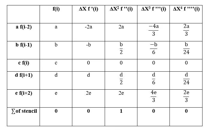
From the above table, we have obtained 5 linear equations,

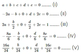
the above equations are solved using the matrix inverse method,

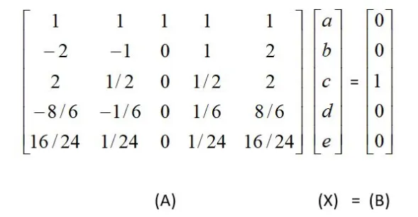
`A X = B`

`X = B A^-1` , we get the values of coefficients as,

a = - 0.0833

b = 1.3333

c = - 2.5000

d = 1.3333

e = - 0.0833

Substituting in the equation gives,

SKEWED RIGHT-SIDED DIFFERENCE SCHEME:

We know that for Skewed right-sided difference scheme,

P = N - Q

Where,

P - The order of accuracy

N - Number of nodes in the stencil

Q - order of derivative

Then, N = P + Q

N = 4 + 2

the Number of nodes, N = 6

Plotting a Symmetric Numeric Stencil with six nodes,

From the above Stencil, for the 2nd order derivative, we get

Using the Taylor Table Method, all the RHS terms in the above equation are expanded using the Taylor Series Method and are represented in the form of a table,

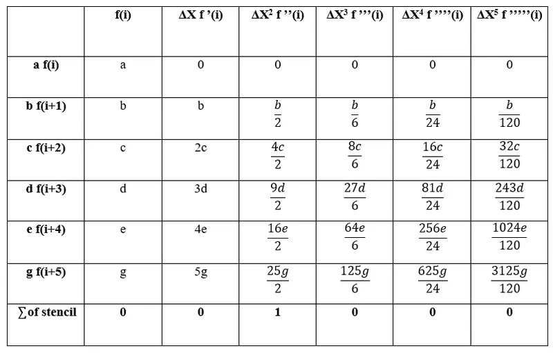
From the above table, we have obtained 6 linear equations,

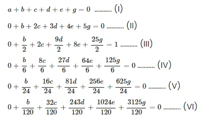
the above equations are solved using the matrix inverse method,

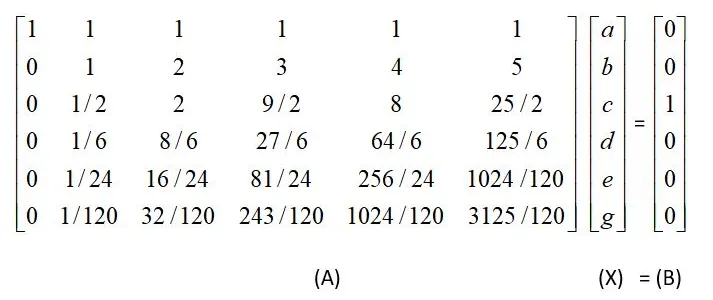
`A X = B`

`X = B A^-1` , we get the values of coefficients as,

a = 3.7500

b = - 12.8333

c = 17.8333

d = - 13.0000

e = 5.0833

g = - 0.8333

Substituting in the equation gives,

SKEWED LEFT-SIDED DIFFERENCE SCHEME:

We know that for Skewed left-sided difference scheme,

P = N - Q

Where,

P - The order of accuracy

N - Number of nodes in the stencil

Q - order of derivative

Then, N = P + Q

N = 4 + 2

the Number of nodes, N = 6

Plotting a Symmetric Numeric Stencil with six nodes,

From the above Stencil, for the 2nd order derivative, we get

Using the Taylor Table Method, all the RHS terms in the above equation are expanded using the Taylor Series Method and are represented in the form of a table,

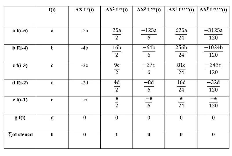
From the above table, we have obtained 6 linear equations,

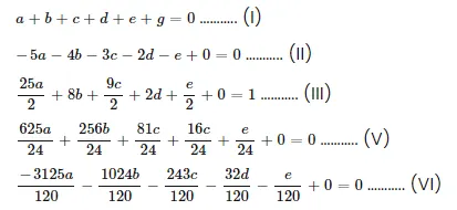
the above equations are solved using the matrix inverse method,

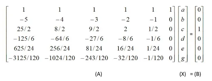
`A X = B`

`X = B A^-1` , we get the values of coefficients as,

a = - 0.8333

b = 5.0833

c = - 13.0000

d = 17.8333

e = - 12.8333

g = 3.7500

Substituting in the equation gives,

Since we know that the truncation error term defines the order of approximation and while applying the values N = 6 and Q = 2 in the thumb rule,

The order of accuracy P = Number of nodes in the stencil N - order of derivative Q

P = 6 - 2

The order of accuracy P = 4

Therefore the skewed schemes are of 4th order accurate.

MATLAB CODES:

FUNCTION CODE FOR CENTRAL DIFFERENCE SCHEME:

function error_central = fourth_order_central_difference (x,dx)

%f(x) = exp(x)*cos(x)

%analytic method 
%f'(x) = exp(x)*cos(x) - exp(x)*sin(x)
%f'' (x) = -2*exp(x)*sin(x)
analytic_method = -2*exp(x)*sin(x);

%numerical method (central differencing)
%coefficient values from taylor table
a = -0.0833;
b = 1.3333;
c = -2.5000;
d = 1.3333;
e = -0.0833;

central_method = ((a*(exp(x-(2*dx))*cos(x-(2*dx))))+(b*(exp(x-dx)*cos(x-dx)))+(c*(exp(x)*cos(x)))+(d*(exp(x+dx)*cos(x+dx)))+(e*(exp(x+(2*dx))*cos(x+(2*dx)))))/(dx^2);

%error
error_central = abs(analytic_method - central_method);

end

FUNCTION CODE FOR SKEWED RIGHT-SIDED DIFFERENCE SCHEME:

function error_skewed_right = fourth_order_skewed_right_difference (x,dx)

%f(x) = exp(x)*cos(x)

%analytic method 
%f'(x) = exp(x)*cos(x) - exp(x)*sin(x)
%f'' (x) = -2*exp(x)*sin(x)
analytic_method = -2*exp(x)*sin(x);

%numerical method (skewed differencing)
%coefficient values from taylor table
a = 3.7500;
b = -12.8333;
c = 17.8333;
d = -13.0000;
e = 5.0833;
g = -0.8333;

right_method = ((a*(exp(x)*cos(x)))+(b*(exp(x+dx)*cos(x+dx)))+(c*(exp(x+(2*dx))*cos(x+(2*dx))))+(d*(exp(x+(3*dx))*cos(x+(3*dx))))+(e*(exp(x+(4*dx))*cos(x+(4*dx))))+(g*(exp(x+(5*dx))*cos(x+(5*dx)))))/(dx^2);

%error
error_skewed_right = abs(analytic_method - right_method);

end

FUNCTION CODE FOR SKEWED LEFT-SIDED DIFFERENCE SCHEME:

MAIN CODE:

%4th order approximation of 2nd order derivative using taylor table method
clear all
close all
clc

%input values
x = pi/3;
dx = linspace(pi/4,pi/4000,20);

for i = 1 : length(dx)
    %function call for central difference scheme
    error_central(i) = fourth_order_central_difference (x,dx(i));
    %function call for skewed right scheme
    error_skewed_right(i) = fourth_order_skewed_right_difference (x,dx(i));
    %function call for skewed left scheme
    error_skewed_left(i) = fourth_order_skewed_left_difference (x,dx(i));

end

%plotting 
figure(1)
loglog(dx,error_central,'linewidth',2)
hold on
loglog(dx,error_skewed_right,'linewidth',2)
loglog(dx,error_skewed_left,'linewidth',2)
xlabel('Range of dx')
ylabel('Truncation Error')
legend('Central Scheme','Skewed Right Scheme','Skewed Left Scheme','location','northwest')

OUTPUT:

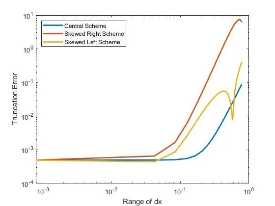
the plot given below compares the absolute error between the three different schemes

CONCLUSION:

• From the plot, the Central Differencing Scheme has the least error value.
• The higher the Truncation Error, the less accurate is the result.
• Thus, the Central Differencing Scheme is better and more accurate than Skewed Schemes.
• The Central Differencing Scheme is accurate as it uses values from both sides of the node considered.

Describe why a skewed scheme is useful? What can a skewed scheme do that a CD scheme cannot?

• In a numerical stencil, if the numerical approximation for a function at the corner node is to be computed, then the Central Differencing Scheme method cannot be used as it requires information from both sides of the node considered.
• As Skewed schemes are useful when there is only information about nodes on one side of the considered node, they can be used for boundary nodes or corner nodes.