OPTIMIZATION OF STALAGMITE USING GENETIC ALGORITHM

Objective:

To optimise the stalagmite function and find the global maxima of the function by using genetic algorithm.

Theory :

Stalagmite:

Stalagmite mathematical model helps to generate local maximas and minimas.

Genetic Algorithm :

Genetic Algorithm is based upon evolution theory proposed by Charles Darwin. This algorithm reflects the process of natural selection where the fittest individuals are selected for reproduction in order to produce offspring of the next generation.

ga in Matlab:

Matlab has inbuilt ga which is used to generate high quality solutions to optimization. ga can be used to solve both constrained and unconstrained optimization problems based on a natural selection process that mimics biological evolution.ga always gets the local minimum value.

Syntax of ga:

1)The general syntax for ga is ,

point=ga(fun,nvars)

which finds a local unconstrained minimum 'point' to the objective function 'fun' and 'nvars' is number of variables.

2)The syntax used here,

[point,fval] = ga(fun,nvars,A,b,Aeq,beq,lb,ub,nonlcon,options)

fun - function to be optimized

nvars - number of variables

A,B - linear inequalities

Aeq,Beq - linear equalities

lb, ub - lower and upper bounds on the design variables

nonlcon - constraints

options - to change the default parameters of ga (used here to change the polulation size of ga)

Stalagmite function code:

function [F]=stalagmite(input_vector)
x=input_vector(1);
y=input_vector(2);
f1x=(sin((5.1*pi*x)+0.5)).^6;
f1y=(sin((5.1*pi*y)+0.5)).^6;
f2x=exp(-4*log(2)*((x-0.0667).^2/0.64));
f2y=exp(-4*log(2)*((y-0.0667).^2/0.64));
F=-(f1x*f1y*f2x*f2y);
end

The ga finds the local minimum by default. To find the global maxima using ga , the negative sign is used for 'F' so that the global maxima becomes local minimum .

Optimimum ga code:

%Stalagmite Mathematical model
clear all
close all
clc
%Defining our search space
x = linspace(0,0.6,150);
y = linspace(0,0.6,150);

%creating a 2Dimensional mesh
[xx,yy]=meshgrid(x,y);

%evaluating the stalagmite function
for i=1:length(xx)
    for j=1:length(yy)
        input_vector(1)=xx(i,j);
        input_vector(2)=yy(i,j);
        f(i,j)=stalagmite(input_vector);
    end
end

%Genetic Algorithm (optimization)

%study 1 : simple ga
tic
no_ga = 50;
for i = 1 : no_ga
[inputs_1(i,:),fval_1(i,:)]=ga(@stalagmite,2);
x_ga(i) = inputs_1(i,1);
y_ga(i) = inputs_1(i,2);
end
%plotting
figure(1)
subplot(2,1,1)
surfc(xx,yy,-f)
title('Study 1')
xlabel('x value')
ylabel('y value')
zlabel('function')
hold on
%to remove grid lines
shading interp
plot3(x_ga,y_ga,-fval_1,'marker','x','markersize',7,'markeredgecolor','red')
subplot(2,1,2)
plot(-fval_1)
xlabel('No of Iteration')
ylabel('Function value')
grid on
opt_fval_1 = -(min(fval_1));
[row, col] = find(fval_1==-(opt_fval_1));
points = inputs_1(row,:);
x_opt_1 = points(1);
y_opt_1 = points(2);
fprintf('\n\n');
o_p = ['Study 1: Global Maxima is f = ',num2str(opt_fval_1) ,' at x = ', num2str(x_opt_1),' , y = ',num2str(y_opt_1)];
disp(o_p);
study_1_time = toc


%study 2 : with boundaries
tic
no_ga = 50;
for i = 1 : no_ga;
[inputs_2(i,:),fval_2(i,:)]=ga(@stalagmite,2,[],[],[],[],[0,0],[0.6,0.6]);
x_ga(i) = inputs_2(i,1);
y_ga(i) = inputs_2(i,2);
end
%plotting
figure(2)
subplot(2,1,1)
surfc(xx,yy,-f)
title('Study 2')
xlabel('x value')
ylabel('y value')
zlabel('function')
hold on
%to remove grid lines
shading interp
plot3(x_ga,y_ga,-fval_2,'marker','x','markersize',7,'markeredgecolor','red')
subplot(2,1,2)
plot(-fval_2)
xlabel('No of Iteration')
ylabel('Function value')
axis([0,50,0,1.5])
grid on
opt_fval_2 = -(min(fval_2));
[row , col] = find(fval_2==-(opt_fval_2));
points = inputs_2(row,:);
x_opt_2 = points(1);
y_opt_2 = points(2);
fprintf('\n\n');
o_p=['Study 2: Global Maxima is f = ',num2str(opt_fval_2) ,' at x = ', num2str(x_opt_2),' , y = ',num2str(y_opt_2)];
disp(o_p)
study_2_time=toc


%study 3 : increased population size
tic
no_ga = 50;
options = optimoptions('ga','PopulationSize',150);
for i= 1 : no_ga
[inputs_3(i,:),fval_3(i,:)] = ga(@stalagmite,2,[],[],[],[],[0,0],[0.6,0.6],[],options);
x_ga(i) = inputs_3(i,1);
y_ga(i) = inputs_3(i,2);
end
%plotting
figure(3)
subplot(2,1,1)
surfc(xx,yy,-f)
title('Study 3')
xlabel('x value')
ylabel('y value')
zlabel('function')
hold on
%to remove grid lines
shading interp
plot3(x_ga,y_ga,-fval_3,'marker','x','color','red','markersize',7,'markeredgecolor','red')
subplot(2,1,2)
plot(-(fval_3))
xlabel('No of Iteration')
ylabel('Function value')
axis([0,50,0.80,1.1])
grid on
opt_fval_3 = -(min(fval_3));
[row,col] = find(fval_3==-opt_fval_3);
point = inputs_3(row,:);
x_opt_3 = points(1);
y_opt_3 = points(2);
fprintf('\n\n');
o_p=['Study 3: Global Maxima is f = ',num2str(opt_fval_3) ,' at x = ', num2str(x_opt_3),' , y = ',num2str(y_opt_3)];
disp(o_p)
study_3_time = toc

• The surface plot is for better understanding of ga for a number of iteration.
• In every study ga is made to run for 50 iterations to note the variation of optimum value generated by ga.
• The optimum study can be determined by the time taken for the study and the accuracy of the study result.

Study 1 - Simple ga :

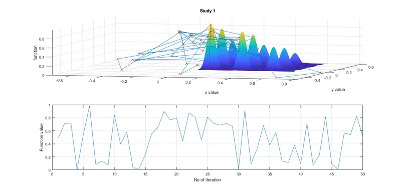
• simple ga has no boundaries and uses default options .
• the heavy variation in function value is because each time ga takes a random set of inputs and runs for the provided stalagmite function.
• so each time ga generates global maxima for that certain set of input .
• more than half of the points lies outside the surface plot which makes this study output unreliable.

The time taken to run the first study always lied between (7 - 22 sec) which is the least of all but yet the results are not accurate.

study 1 (simple ga) has poor accuracy with fastest time .

Study 2 - ga with boundaries :

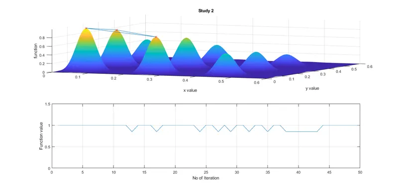
• the addition of lower and upper boundary conditions made ga more intresting by considerably reducing the variation of global maxima generated by ga for different iterations.
• still ga tends to go for local maxima more which makes the ouput of this study less relaiable.

This study always took time of (11-30 sec) which is far better considering the accuracy of the generated results. But still the accuracy of output is needed to be increased.

study 2 (ga with boundaries) has better accuracy taking some more time .

Study 3 - ga with optimised population size :

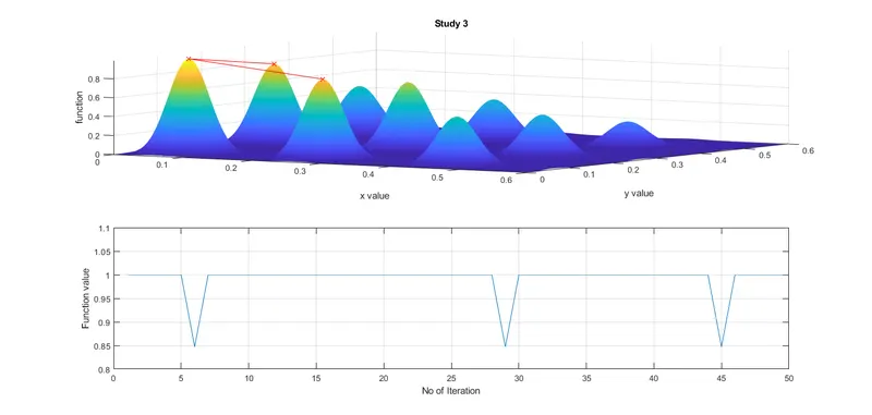
• the ga is used with upper and lower boundaries and increased population size.
• the ga input population size is increased from 50 (default) to 150 by using optimoption function to increase the accuracy.
• comparing with the above studies, this study has the precised output values.

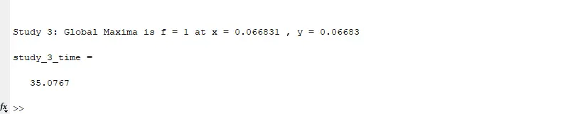
the time taken for this study is always more than 30sec which makes it the slowest study of all but still the accuracy of the output is best of all studies.

study 3 (ga with increased population size) has the best accuracy of all making it the slowest .

Result:

The stalagmite function is successfully optimised and global maxima is found using ga.