Week 9 - FVM Literature Review
FVM Literature Review
Finite Volume Method(FVM):
The finite volume method (FVM) is a discretization technique for partial differential equations, especially those that arise from physical conservation laws. FVM uses a volume integral formulation of the problem with a finite partitioning set of volumes to discretize the equations. FVM is in common use for discretizing computational fluid dynamics equations.
The mathematical foundation of the FVM is the Gauss integral theorem.
`∮_V(Δ.vec a)dV=∮_sveca.hat n ds`
`veca:`generic vector
`hat n:`the outer normal to the surface
The Finite Volume Method (FVM) is one of the most versatile discretization techniques used in CFD. Based on the control volume formulation of analytical fluid dynamics, the first step in the FVM is to divide the domain into a number of control volumes (i.e. cells, elements) where the variable of interest is located at the centroid of the control volume. The next step is to integrate the differential form of the governing equations (very similar to the control volume approach) over each control volume.
Interpolation profiles are then assumed in order to describe the variation of the concerned variable between cell centroids. The resulting equation is called the discretized or discretization equation. In this manner, the discretization equation expresses the conservation principle for the variable inside the control volume.
The most compelling feature of the FVM is that the resulting solution satisfies the conservation of quantities such as mass, momentum, energy, and species. This is exactly satisfied for any control volume as well as for the whole computational domain and for any number of control volumes. Even a coarse grid solution exhibits exact integral balances.
FVM is the ideal method for computing discontinuous solutions arising from incompressible flows. Any discontinuity must satisfy the Rankine-Hugoniot jump condition which is a consequence of conservation. Since finite volume methods are conservative they automatically satisfy the jump conditions and hence give physically correct weak solutions.
FVM is also preferred while solving partial differential equations containing discontinuous coefficients.
The major differences between FDM & FVM:
| FDM | FVM |
| Governing equations are in the differential form. | Governing equations are in the integral form. |
| The domain is divided into points with each point representing a variable of interest. (that are grid points) | The domain is divided into control volumes or cells with variables of interest located at the centroid of each control volume. |
| Structured grids in most cases, difficult for complex geometry. | Structured and unstructured grids as the shape of control volume do not impact conservation principles. |
| Easy to obtain higher order schemes,so preferable for applications that require very high accuracy. | Deriving schemes higher than second order is next to impossible due to the complexity involved. |
| Unsuitable for handling discontinuities. | Can handle discontinuities,due to nature of integral equation. |
| Conservation laws are not preserved in all cases. | Conservation principles including mass, momentum and energy are maintained by definition. |
FDM FVM
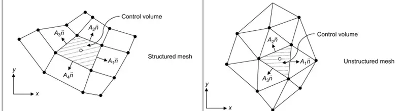
The need for interpolation schemes in FVM:
Consider the 1D Heat Conduction Equation:
`del/(delx)(alpha*(delT)/(delx))+S=0`(i)
Where S=source term
`alpha=`thermal diffusivity
`(delT)/(delx)=` temperature gradient along the x direction
Governing equation is valid at every point in domain, which means it is also valid in entire control volume.
If small control volume (dv) is considered and it is multiplied with the governing equation and integrated it for entire volume then that should be also equal to zero i.e the 'integral form of governing equation'.
Taking the conservation equation validated at single point and if it is validated at single point then it is validated at entire volume and in this entire volume properties are conserved.
Multiplying the equation by 'dv' and integrating it
`int(del/(delx)(alpha.(delT)/(delx))+S) dv = 0`
`int(del/(delx)(alpha.(delT)/(delx))dv+ intS dv = 0`
`because dv = A .dx`
`intdel/(delx)(alpha.(delT)/(delx))A.dx+ intS dv = 0`
`[alphaA((delT)/(delx))]_w^e +overlineS dv = 0`
S is average value of source term (S) which when multiplied by dv is going to be equal to `intS dv`
`alpha_eA(delT)/(delx_e)-alpha_wA(delT)/(delx_w) +overlineS dv = 0`
If we assume α as a constant and not a function of temperature,
`alpha A[(T_E-T_P)/(Deltax)]-alphaA[(T_P-T_W)/(Deltax)] + overlineSdv =0`
The source term which is to be added in a cell, if it is a function of temperature we have to linearize it.
if `alpha`is a function of temperature we have to linearize it.
`(overline S underline("linearization") to S_u+S_pT_p)`
`alpha A[(T_E-T_P)/(Deltax)]-alphaA[(T_P-T_W)/(Deltax)] + overlineSdv =0`
`[Heat flux]_("out")-[Heat flux]_("in")+Source term =0`
The amount of heat that is removed from a particular box is conserved.
Different schemes are used to solve the equation:
1. Gradient scheme
2. Interpolation scheme
Interpolation scheme:
In the finite volume formulation, evaluation of surface and volume integrals sometimes requires the values of unknown variables at locations other than the computational nodes of the control volume. These values are obtained by employing certain interpolation schemes.
To calculate `T_w`and `T_e`Temperature at the west and east faces, we have the value at `T_P, T_E, and T_W`by interpolating the values, we can get the temperature at the east and west faces. By using them we can calculate the thermal diffusivity of the faces are `alpha_e and alpha_w`
here are different ways of Interpolation. Some of the ways are given by
- Upwind Interpolation scheme.
- Linear Interpolation scheme.
- Quadratic Interpolation scheme.
- Hybrid Interpolation Scheme.
Upwind Interpolation scheme :
The upwind interpolation scheme (UDS) for approximating the value of a variable f at the east face of a control volume is given by
`f_e= {(f_(p ) if (v.n)_e>0),(f_E if (v.n)_e<0):}`
This interpolation scheme is essentially equivalent to using the forward difference method or backward difference method depending on the flow direction. Here, the direction of velocity at a given point determines the variable value to be used in an interpolation process. As the name suggests, we use the node upwind or upstream from the given node.
Upwind interpolation is the only approximation that satisfies the boundedness criterion unconditionally in the sense that irrespective of the velocity values and grid spacing, the solution will always remain bounded. This is the use of upwind interpolation which will never yield oscillatory solutions.
t is generally used convection-dominated problems (i.e pe >1).
The values of the interface is given by:
for v > 0, we have
`u_(i-1/2) approx u_(i-1) , u_(i+1/2) approx u_(i)`
`I_c approx v {u_i - u_(i-1)}/{Deltax}`Backward difference
for v < 0, we have
`u_(i-1/2) approx u_(i) , u_(i+1/2) approx u_(i+1)`
`I_c approx v {u_(i+1) - u_i}/{Deltax}`Forward difference
Linear Interpolation Scheme:
The approximated value of the variable at control volume centroid by linear interpolation of the values at two nearest computational nodes.
`f_e = f_E lambda_e + f_p(1-lambda_e)`
where `lambda_e = {x_e - x_p}/{x_E-x_p}`
The linear interpolation is equivalent to the use of the CDS formula of the first-order derivative, and hence this scheme is also termed as Central Differencing Scheme(CDS). This is 2nd-order accurate and may produce oscillatory results therefore small grids are preferred for this method. This is one of the most widely used interpolation methods.
Quadratic Interpolation scheme:
The approximated values of the variable at the control volume's centroid by quadratic interpolation of the values at the three nearest computational nodes which consist of one downstream node 'D' and two upstream nodes 'UU'.It is third order accurate for both uniform and nonuniform grids.
`f_e = f_U + g_1(f_D - f_U) + g_2(f_(UU) -f_u)`
`g_1 = {(x_e - x_U)(x_e - x_(UU))}/{(x_D - x_U)(x_D-x_(UU))`
`g_2 = {(x_e - x_U)(x_e - x_D)}/{(x_(UU) - x_D)(x_(UU)-x_(U))`
The relation obtained as:
`phi_e = 6/8phi_c + 3/8phi_D - 1/8phi_(UU)`
Hybrid Interpolation Scheme:
It is the blend of CDS and UDS schemes, based on the Peclet number.
`f_e = gammaf_(CDS) + (1-gamma)f_(UDS)`
Flux Limiters
While calculating the variable gradients they tend to toggle and are not bounded to a particular value and keep jumping, this occurs due to discontinuity due to shock occuring , having a flux limiter will help to bound the gradient value thereby giving a stable solution.
Numerical approximation using higher order spatial discretization schemes results in better accuracy but exhibits spurious oscillations near discontinuities such as shocks. On the other hand, lower order spatial discretization schemes remain stable near discontinuities but dampen out the distributions because of their dissipative nature. Hence in order to capture discontinuities, high resolution schemes are desired - which are highly accurate and stable throughout the domain.
Flux limiters operate functionally as a switch and tune the numerical fluxes obtained from lower order scheme and higher order scheme such that near the discontinuity lower order (stable) scheme is employed and away from it higher order (accurate) scheme is employed.
`H_e`represents flux at e calculated using higher order scheme
`L_e`represents flux at e calculated using lower order scheme
`psi(r)` represents flux limiter function
`F_e = L_e + psi(r)(H_e-L_e)`
Flux limiter function depends upon the smoothness parameter r which is defined as:
`r_P = (phiP-phiW)/(phiE-phiP)`
The flux limiter function is constrained to be greater than or equal to zero. It assumes a value of 0 near discontinuities and a value of 1 away from them. Hence it switches between higher order scheme and lower order scheme for numerical representation of flux, thereby keeping the scheme stable and accurate throughout.
Note that flux limiters are also referred to as slope limiters because they both have the same mathematical form, and both have the effect of limiting the solution gradient near shocks or discontinuities. In general, the term flux limiter is used when the limiter acts on system fluxes and slope limiter is used when the limiter acts on system states (like pressure, velocity etc.).
consider 1D- semi-discrete scheme
`(du_i)/(dt)+1/(Deltax_i)[F(u_(i+1/2)) - F(u_(i-1/2))] = 0`
`F(u_(i+1/2)) & F(u_(i-1/2))`
`F(u_(i+1/2)) = f_(i+1/2)^(low) - phi(ri)(f_(i+1/2)^(low)-f_(i+1/2)^(high))`
`F(u_(i-1/2)) = f_(i-1/2)^(low) - phi(ri)(f_(i-1/2)^(low)-f_(i-1/2)^(high))`
Where
`f^(low)` =low resolution flux,
`f^(high)` =high resolution flux,
`phi(r)` =flux limiter function.
where r represents the ratio of successive gradients on the solution mesh,
`phi(r)ge 0`
this is the limiter function case
if limiter function = 0 , then there will be a low resolution and sharp gradient.
if limiter function > 0 , then there will be a high resolution and +ve gradient.