Week 3 - Solving second order ODEs

The equation (ODE ) of motion of a simple pendulum with damping

AIM:

To write a program in MATLAB that solves the ODE of the simple pendulum with damping.

GOVERNING EQUATION:

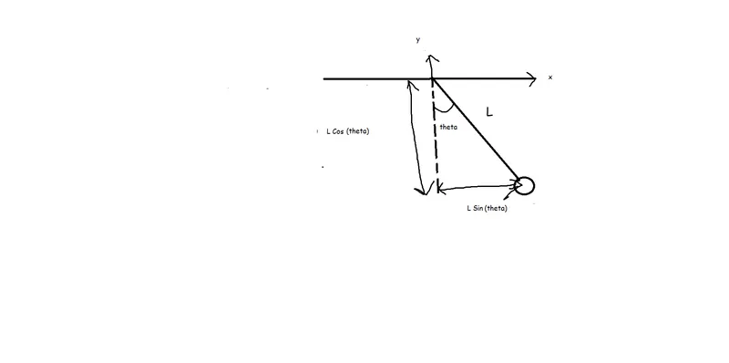
Θ= Θ₁

_d Θ/ dt = _d Θ_1/dt ₌ Θ₂

_d² Θ/ dt² = _d² Θ_1/ dt²_{= d/dt (d} Θ_1/ dt_{) = d /}dt(Θ₂)

_d² Θ_1/ dt²+b/m(_d Θ_1/dt)+g/Lsin Θ₁=0

_d Θ_2/dt+ b/m (Θ₂)+ g/Lsin Θ₁=0

_d Θ_2/dt=- b/m (Θ₂)- g/Lsin Θ₁

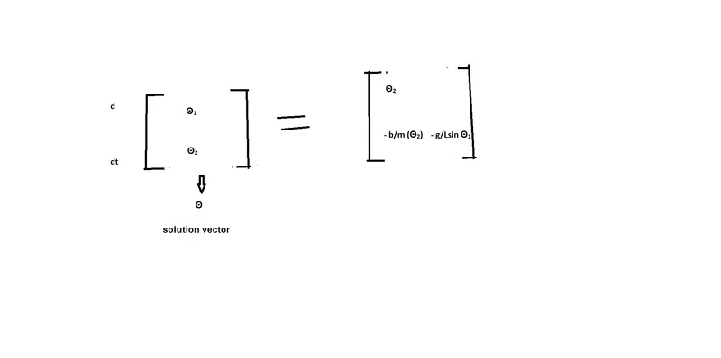
Where,

g = gravity ( m/s2)

L = length of the pendulum (m)

m = mass of the ball (kg)

b=damping coefficient.

The way the pendulum moves depends on Newton's second law. When this law is written down, we get a second-order Ordinary Differential Equation that describes the position of the "ball" w.r.t time.

Objectives:

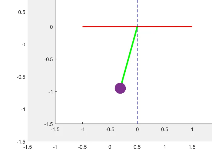
1. To create an image that represents the position of the pendulum.

2. To create an animation to show the motion of the pendulum.

PROCEDURE:

clear all
close all
clc

%inputs(length of pendulam,mass,damping coefficient,gravity)
L=1;
m=1;
b=0.05;
g=9.81;

% initial condition ( displacement,angular velocity)(at t=0)
theta_0=[0,3];

%time points
t_span=linspace(0,20,500);

%solve ODE
[t,results]=ode45(@(t,theta) ode_func(t,theta,b,g,L,m),t_span,theta_0);

%plotting
plot(t,results(:,1),'color','r')
hold on
grid on
plot (t,results(:,2),'color','g')
ylabel('plot')
xlabel('time')
legend('displacement','angular velocity')

%animation

ct=1
for i=1:length(results(:,1));
  
    x0=0;
    y0=0;
    x1=L*sin(results(i,1));
    y1=-L*cos(results(i,1));

    %plotting
    plot([-1 1],[0 0],'LineWidth',2,'Color','r');
    hold on
    plot([0 0],[-1.5 .5],'LineStyle','--','Color','b');
    %length of string
    plot([x0 x1],[y0 y1],'LineWidth',3,'Color','g');
    hold on
    %ball of the pendulum
    plot(x1,y1,'.','MarkerSize',75);
    
    axis([-1.5 1.5 -1.5 0.5])
    hold off
    pause(0.001)
    M(ct)=getframe(gcf);
    ct=ct+1;
end

movie(M)
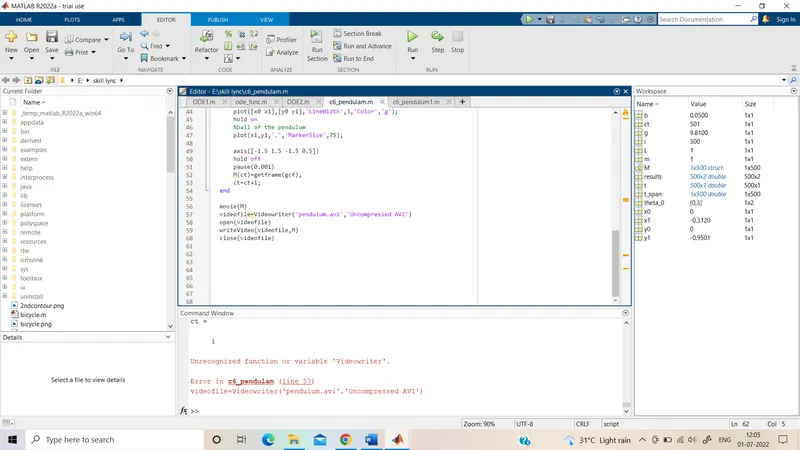
videofile=VideoWriter('pendulum.avi','Uncompressed AVI')
open(videofile)
writeVideo(videofile,M)
close(videofile)

    

STEP-I Clear all (to clear all the stored data to a variable, close all (to close all Matlab fig. window),clc (to clear the command window) commands are used.

STEP-II Inputs are given

L=1 meter,

m=1 kg,

b=0.05.

g=9.81 m/s2.

STEP-III

STEP-IV

Time span is inputted using linspace command

for 0-20 sec (500 values)

STEP-V

A numerical ODE solver is used as the main tool to solve the ODE. The Matlab function ode45 is used. The important thing to remember is that ode45 can only solve a first order ODE. Therefore to solve a higher-order ODE, the ODE has to be first converted to a set of first order ODE.

calling the ode function which is created separately.

function [dtheta_dt]=ode_func(t,theta,b,g,L,m)

theta1=theta(1)
theta2=theta(2)
dtheta1_dt=theta2;
dtheta2_dt=-(b/m)*theta2-(g/L)*sin(theta1);
dtheta_dt=[dtheta1_dt;dtheta2_dt];
end

STEP-VI

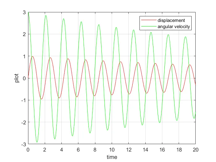
Plotting time vs displacement and angular velocity

results(:,1) displacement

results(:,2)angular velocity

STEP-VII

Creating animation

for loop is used to show the movement of the ball.

The length of the string and the size of the ball is assumed.

marker command has been used to create the sphere.

OUTPUTS:

time vs. displacement and velocity plot

position of pendulum

https://youtu.be/6-w1PdZg-Io

ERRORS:

ERROR1:While creating Ode func inputted l instead of L( Length of the pendulum)

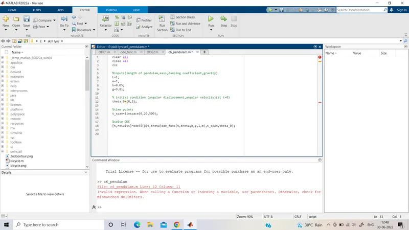
REMEDY1:In ode fuction Length of the pendulum is changed as L . Error 1 resolved.

ERROR2:Problem while creating the video file

REMEDY2: