Project 1 - Parsing NASA thermodynamic data
Project 1 - Parsing NASA thermodynamic data
AIM: To write a code in MATLAB for parsing the NASA thermodynamic data file and then calculate the thermodynamic properties of various species.
OBJECTIVES:
1. To write a function that extracts the 14 coefficients and calculates the enthalpy, entropy, and specific heats for all the species in the data file.
2. To Calculate the molecular weight of each species and display it in the command window.
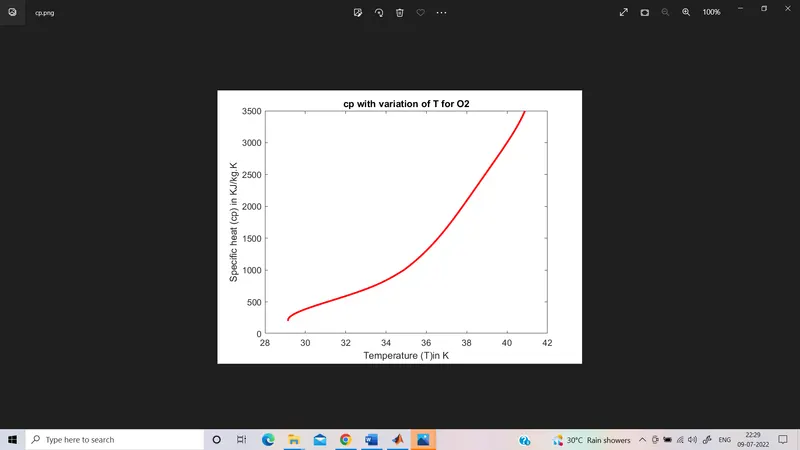
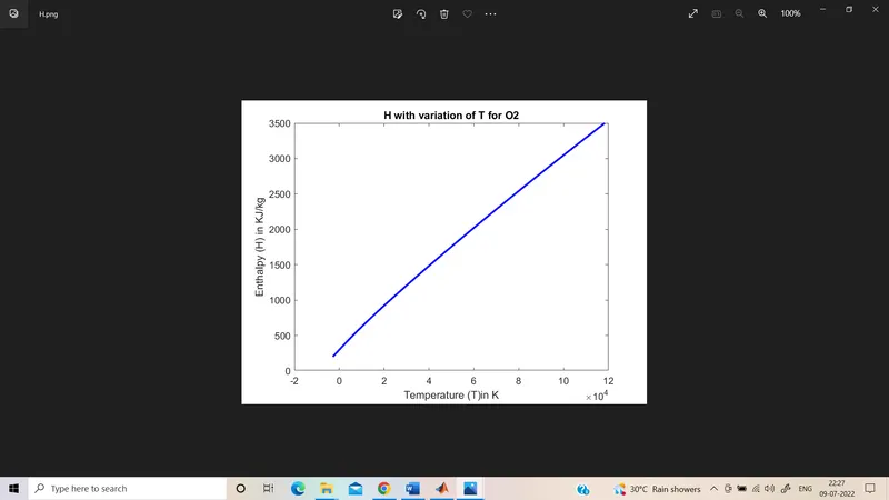
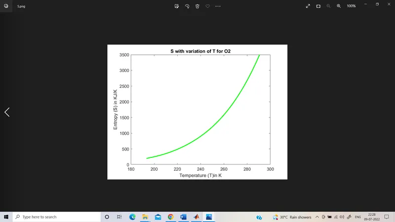
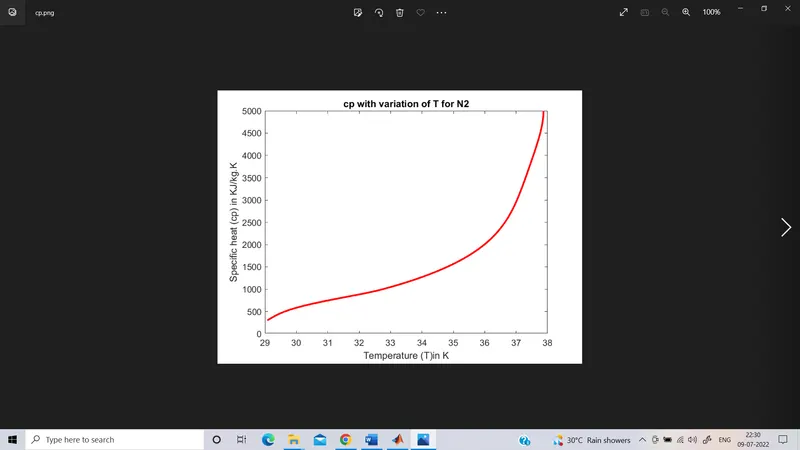
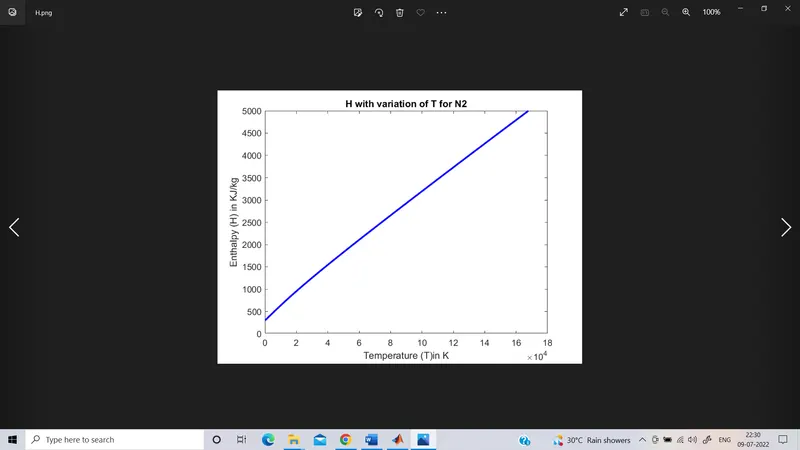
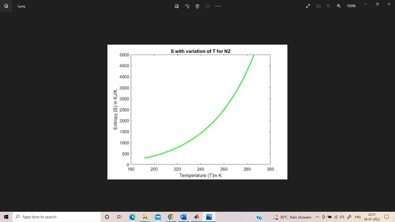
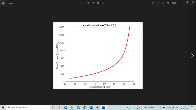
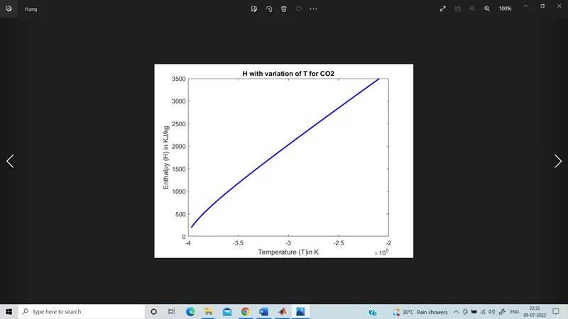
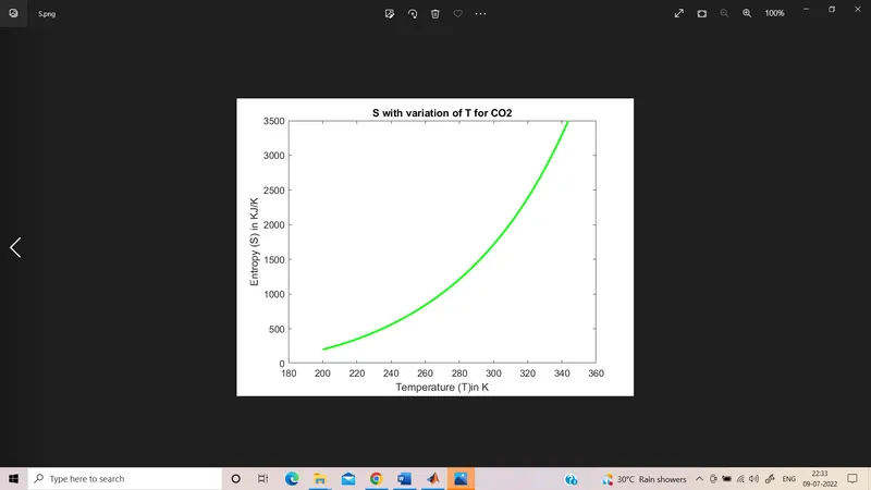
3. To plot the Cp, Enthalpy, and Entropy for the local temperature range (low temperature: high temperature) specific for each species.
4. To save the plots as images with appropriate names and dump them in separate folders for each species with a suitable name.
THEORY:
Parsing in computer languages refers to the syntactic analysis of the input code into its components parts in order to facilitate the writing of compilers and interpreters. It can be used to describe split or separation.
Parsing a file means reading in a data stream of some sort and building an in-memory model of the semantic content of that data. This aims at facilitating performing some kind of transformation on the data.
GOVERNING EQUATIONS:
The formulas used are shown below.
Here R is the universal gas constant;
R = 8.3144598(48) J⋅mol^−1⋅K^−1., T is the temperature.
cp=specific heat
S=entropy
H=enthalpy
The FIRST 7 coefficients are HIGH-temperature coefficients and the SECOND 7 coefficients are LOW-temperature coefficients.
a1-a7=high temperature coefficient
a8-a14=low temperature coefficient
BASIC PROGRAMMING:
clear all
close all
clc

%  Nasa thermodynamic file parsing

f1=fopen('THERMO.dat','r');
fgetl(f1)

%reading the header information
tline1=fgetl(f1);
A=strsplit(tline1,' ');

%global temp
Global_low_temp=str2num(A{2});
Global_mid_temp=str2num(A{3});
Global_high_temp=str2num(A{4});

%skipping the next three lines
for i = 1:3
    skippinglines = fgetl(f1);
end
%reading species block
for i=1:53

header=fgetl(f1);
    x=strsplit(header,' ');

    species_name=(x{1});
    z=length(x);

local_low_temp=str2double(x{z-3});
        local_high_temp=str2double(x{z-2});
            local_mid_temp=str2double(x{z-1});

           T1=local_low_temp;
           T2=local_mid_temp;
           T3=local_high_temp;

%getting line_1 coeffecients (a1-a5)
tline_1=fgetl(f1);
a=strfind(tline_1,'E');
a1=tline_1(1:a(1)+3);
a1=str2num(a1);
a2=tline_1(a(1)+4:a(2)+3);
a2=str2num(a2);
a3=tline_1(a(2)+4:a(3)+3);
a3=str2num(a3);
a4=tline_1(a(3)+4:a(4)+3);
a4=str2num(a4);
a5=tline_1(a(4)+4:a(5)+3);
a5=str2num(a5);

%getting line_2 coeffecients (a6-a10)
tline_2=fgetl(f1);
a=strfind(tline_2,'E');
a6=tline_2(1:a(1)+3);
a6=str2num(a6);
a7=tline_2(a(1)+4:a(2)+3);
a7=str2num(a7);
a8=tline_2(a(2)+4:a(3)+3);
a8=str2num(a8);
a9=tline_2(a(3)+4:a(4)+3);
a9=str2num(a9);
a10=tline_2(a(4)+4:a(5)+3);
a10=str2num(a10);

%getting line_3 coeffecients (a11-a14)
tline_3=fgetl(f1);
a=strfind(tline_3,'E');
a11=tline_3(1:a(1)+3);
a11=str2num(a11);
a12=tline_3(a(1)+4:a(2)+3);
a12=str2num(a12);
a13=tline_3(a(2)+4:a(3)+3);
a13=str2num(a13);
a14=tline_3(a(3)+4:a(4)+3);
a14=str2num(a14);

%reading the species

T = linspace(T1,T3,100);
R = 8.314;

% specific heat(cp), Entahlpy(H) and Entropy(S) calculation
for i=1:length(T)
    if T(i)>T2
        cp(i)=R*(a1+a2.*T(i)+a3.*T(i).^2+a4.*T(i).^3+a5.*T(i).^4);
        H(i)= R*T(i).*(a1+((a2*T(i)/2))+((a3*T(i).^2)/3)+((a4*T(i).^3)/4)+((a5*T(i).^4)/5)+((a6./T(i))));
        S(i)= R*(a1.*log(T(i))+a2.*T(i)+a3.*(T(i)^2)/2+a4.*(T(i)^3)/3+a5.*(T(i)^4)/4+a7);
    else
        cp(i)=R*(a8+a9.*T(i)+a10.*T(i).^2+a11.*T(i).^3+a12.*T(i).^4);
        H(i)= R*T(i).*(a8+((a9*T(i)/2))+((a10*T(i).^2)/3)+((a11*T(i).^3)/4)+((a12*T(i).^4)/5)+((a13./T(i))));
        S(i)= R*(a8.*log(T(i))+a9.*T(i)+a10.*(T(i)^2)/2+a11.*(T(i)^3)/3+a12.*(T(i)^4)/4+a14);
    end
end


%folder creating
mkdir(species_name)
cd(species_name)


%plotting cp with variation of T
figure(1)
plot(cp,T,'LineWidth',2,'color','r')
xlabel('Temperature (T)in K')
ylabel('Specific heat (cp) in KJ/kg.K')
title(sprintf('cp with variation of T for %s',species_name))
saveas(figure(1),'cp.png')

%plotting H with variation of T
figure(2)
plot(H,T,'LineWidth',2,'color','b')
xlabel('Temperature (T)in K')
ylabel('Enthalpy (H) in KJ/kg')
title(sprintf('H with variation of T for %s',species_name))
saveas(figure(2),'H.png')

%plotting S with variation of T
figure(3)
plot(S,T,'LineWidth',2,'color','g')
xlabel('Temperature (T)in K')
ylabel('Entropy (S) in KJ/K')
title(sprintf('S with variation of T for %s',species_name))
saveas(figure(3),'S.png')
cd ..

% Calculating the molecular weight
[molecularweight]=mw(species_name);
fprintf('the molecular weight of %s is %d\n',species_name,molecularweight)

 end
STEPS:
- Clear all (to clear all the stored data to a variable, close all (to close all Matlab fig. window),clc (to clear the command window) commands are used.
- A suitable program name is given.
- To read the data file fopen command is used, and to get the information fgetl is used.
- To read the header information tline1=fgetl(f1) is used.
- Using strsplit we are able to split the string .
- The global temperatures ( low, mid, and high) are fetched using str2num.
- By creating for loop i = 1:3 and using fgetl(f1)we are able to skip the next three lines which are not required.
- To read the species block (53) for loop command is created.
- To read the header strsplit and to read the local temperatures str2double is used.
T1=local_low_temp;T2=local_mid_temp;T3=local_high_temp;
- To get temperature coefficient values we used strfind to specify them accurately. So the data is in string format in order to convert it into a number str2num is used.
- To calculate specific heat(cp), Enthalpy(H) and Entropy(S) for loop ,if-else logic created.
- To plot, we need a set of temperatures so linspace is used to split the local temperatures into 100 divisions.
- mkdir command is used to make a directory.The directory is the folder where MATLAB looks for all the components of code.
- cd prints out the current directory.
- plotting of Cp, Enthalpy, and Entropy with temperature is done using the plot command .
- cd.. is used to save all the plots for different species.
- Molecular weight is calculated by calling a function mw.m
-
function[molecularweight]=mw(species_name)

elements = ['H','C','O','N','A'];
atomic_weight=[1,12,16,14,40];
molecularweight=0;
for i=1:length(species_name)
for j=1:length(elements)
if strcmpi(species_name(i),elements(j))
 molecularweight = molecularweight+atomic_weight(j) ;

%Storing the position of matched element
                position = j;
         end
end
 end
  n = str2double(species_name(i));
       if(n>1)
 molecularweight =molecularweight+(atomic_weight(position)*(n-1));
       end


end
-
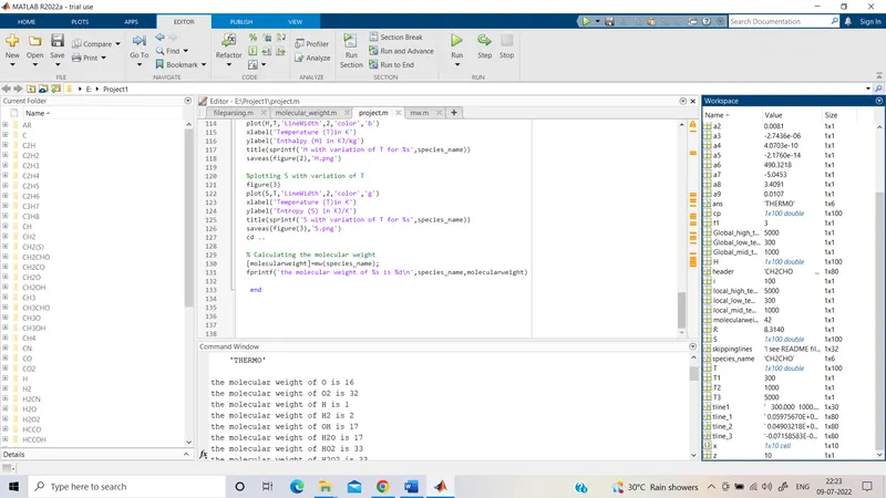
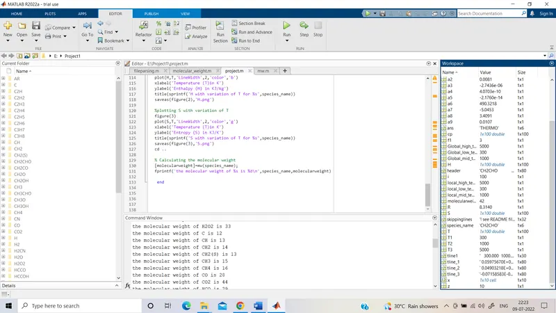
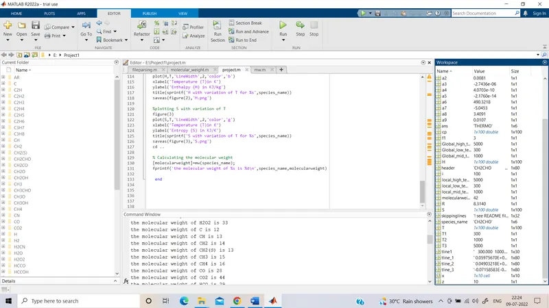
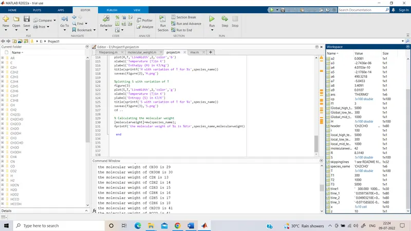
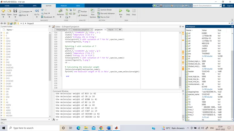
By using fprintf the molecular weight of each species is displayed in the command window.the molecular weight of O is 16
the molecular weight of O2 is 32
the molecular weight of H is 1
the molecular weight of H2 is 2
the molecular weight of OH is 17
the molecular weight of H2O is 17
the molecular weight of HO2 is 33
the molecular weight of H2O2 is 33
the molecular weight of C is 12
the molecular weight of CH is 13
the molecular weight of CH2 is 14
the molecular weight of CH2(S) is 13
the molecular weight of CH3 is 15
the molecular weight of CH4 is 16
the molecular weight of CO is 28
the molecular weight of CO2 is 44
the molecular weight of HCO is 29
the molecular weight of CH2O is 29
the molecular weight of CH2OH is 30
the molecular weight of CH3O is 29
the molecular weight of CH3OH is 30
the molecular weight of C2H is 13
the molecular weight of C2H2 is 14
the molecular weight of C2H3 is 15
the molecular weight of C2H4 is 16
the molecular weight of C2H5 is 17
the molecular weight of C2H6 is 18
the molecular weight of CH2CO is 41
the molecular weight of HCCO is 41
the molecular weight of HCCOH is 42
the molecular weight of H2CN is 27
the molecular weight of HCN is 27
the molecular weight of HNO is 31
the molecular weight of N is 14
the molecular weight of NNH is 29
the molecular weight of N2O is 30
the molecular weight of NH is 15
the molecular weight of NH2 is 16
the molecular weight of NH3 is 17
the molecular weight of NO is 30
the molecular weight of NO2 is 46
the molecular weight of HCNO is 43
the molecular weight of HOCN is 43
the molecular weight of HNCO is 43
the molecular weight of NCO is 42
the molecular weight of CN is 26
the molecular weight of HCNN is 41
the molecular weight of N2 is 28
the molecular weight of AR is 40
the molecular weight of C3H8 is 20
the molecular weight of C3H7 is 19
the molecular weight of CH3CHO is 42
the molecular weight of CH2CHO is 42