Week 4.1 - Genetic Algorithm

Genetic Algorithm

Aim: To write a code in MATLAB to optimise the stalagmite function and find the global maxima of the function.

Objectives:

• To explain the concept of genetic algorithm and the syntax for ga in MATLAB
• Plot graphs for all 3 studies and for F maximum vs no. of iterations.

Genetic Algorithm(GA)– Fundamentals:

Genetic Algorithm (GA) is a search-based optimization technique based on the principles of Genetics and Natural Selection. It is frequently used to find optimal or near-optimal solutions to difficult problems which otherwise would take a lifetime to solve. It is frequently used to solve optimization problems, in research, and in machine learning.

Optimization:

Optimization refers to finding the values of inputs in such a way that we get the “best” output values.

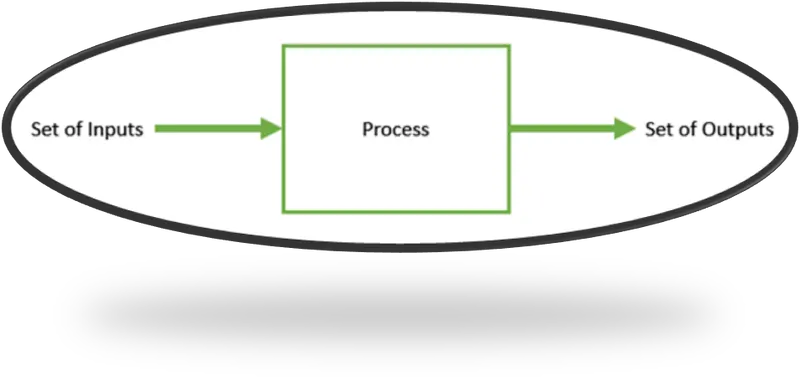
Optimization

Basic Terminology

Before beginning a discussion on Genetic Algorithms, it is essential to be familiar with some basic terminology :

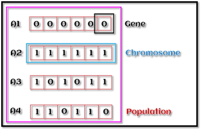
• Population− It is a subset of all the possible (encoded) solutions to the given problem. The population for a GA is analogous to the population for human beings except that instead of human beings, we have Candidate Solutions representing human beings.
• Chromosomes− A chromosome is one such solution to the given problem.
• Gene− A gene is one element position of a chromosome.
• Allele− It is the value a gene takes for a particular chromosome.
• Fitness Function-The fitness function is used to determine the individual's fitness level in the population. It means the ability of an individual to compete with other individuals. In every iteration, individuals are evaluated based on their fitness function.
• Genetic Operators-In a genetic algorithm, the best individual mate to regenerate offspring better than parents. Here genetic operators play a role in changing the genetic composition of the next generation.
• Selection-After calculating the fitness of every existent in the population, a selection process is used to determine which of the individualities in the population will get to reproduce and produce the seed that will form the coming generation.

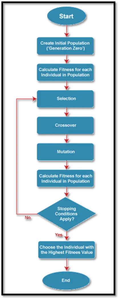
The genetic algorithm works on the evolutionary generational cycle to generate high-quality solutions. These algorithms use different operations that either enhance or replace the population to give an improved fit solution.

It basically involves five phases to solve the complex optimization problems, which are given below:

• Initialization: The process of a genetic algorithm starts by generating a set of individuals, which is called a population. Here each individual is the solution to the given problem. An individual contains or is characterized by a set of parameters called Genes. Genes are combined into a string and generate chromosomes, which is the solution to the problem. One of the most popular techniques for initialization is the use of random binary strings.

• Fitness Assignment: The fitness function is used to determine how fit an individual is? It means the ability of an individual to compete with other individuals. In every iteration, individuals are evaluated based on their fitness function. The fitness function provides a fitness score to each individual. This score further determines the probability of being selected for reproduction. The high the fitness score, the more chances of getting selected for reproduction.
• Selection: The selection phase involves the selection of individuals for the reproduction of offspring. All the selected individuals are then arranged in a pair of two to increase reproduction. Then these individuals transfer their genes to the next generation.

  There are three types of Selection methods available, which are:

  • Roulette wheel selection
  • Tournament selection
  • Rank-based selection
• Reproduction: After the selection process, the creation of a child occurs in the reproduction step. In this step, the genetic algorithm uses two variation operators that are applied to the parent population. The two operators involved in the reproduction phase are given below:

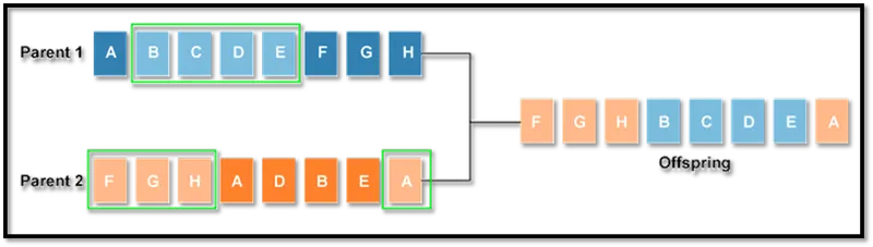
Crossover: The crossover plays a most significant role in the reproduction phase of the genetic algorithm. In this process, a crossover point is selected at random within the genes. Then the crossover operator swaps the genetic information of two parents from the current generation to produce a new individual representing the offspring.
The genes of parents are exchanged among themselves until the crossover point is met. These newly generated offspring are added to the population. This process is also called crossover. Types of crossover styles available:

• One point crossover
• Two-point crossover
• Livery crossover
• Inheritable Algorithms crossover

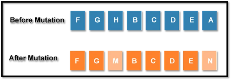
Mutation: The mutation operator inserts random genes in the offspring (new child) to maintain the diversity in the population. It can be done by flipping some bits in the chromosomes.
Mutation helps in solving the issue of premature convergence and enhances diversification. The below image shows the mutation process:
Types of mutation styles available,

• Flip bit mutation
• Gaussian mutation
• Exchange/Swap mutation

Termination: After the reproduction phase, a stopping criterion is applied as a base for termination. The algorithm terminates after the threshold fitness solution is reached. It will identify the final solution as the best solution for the population.

General Workflow of a Simple Genetic Algorithm:

Advantages:

• The parallel capabilities of genetic algorithms are best.
• It helps in optimizing various problems such as discrete functions, multi-objective problems, and continuous functions.
• It provides a solution for a problem that improves over time.
• A genetic algorithm does not need derivative information.

Limitations:

• Genetic algorithms are not efficient algorithms for solving simple problems.
• It does not guarantee the quality of the final solution to a problem.
• Repetitive calculation of fitness values may generate some computational challenges.

GA in MATLAB :Find minimum of function using genetic algorithm but in this case we have to find maximum.

SYNTAX

x = ga(fun,nvars,A,b) finds a local minimum x to fun, subject to the linear inequalities A*x ≤ b. ga evaluates the matrix product A*x as if x is transposed (A*x').

x = ga(fun,nvars,A,b,Aeq,beq) finds a local minimum x to fun, subject to the linear equalities Aeq*x = beq and A*x ≤ b. (Set A=[] and b=[] if no linear inequalities exist.) ga evaluates the matrix product Aeq*x as if x is transposed (Aeq*x').

x = ga(fun,nvars,A,b,Aeq,beq,lb,ub) defines a set of lower and upper bounds on the design variables, x, so that a solution is found in the range lb ≤ x ≤ ub. (Set Aeq=[] and beq=[] if no linear equalities exist.)

x = ga(fun,nvars,A,b,Aeq,beq,lb,ub,nonlcon) subjects the minimization to the constraints defined in nonlcon. The function nonlcon accepts x and returns vectors C and Ceq, representing the nonlinear inequalities and equalities respectively. ga minimizes the fun such that C(x) ≤ 0 and Ceq(x) = 0. (Set lb=[] and ub=[] if no bounds exist.)

x = ga(fun,nvars,A,b,Aeq,beq,lb,ub,nonlcon,options) minimizes with the default optimization parameters replaced by values in options. (Set nonlcon=[] if no nonlinear constraints exist.) Create options using optimoptions.

x = ga(fun,nvars,A,b,Aeq,beq,lb,ub,nonlcon,intcon) or x = ga(fun,nvars,A,b,Aeq,beq,lb,ub,nonlcon,intcon,options) requires that the variables listed in intcon take integer values.

x = ga(problem) finds the minimum for problem, a structure described in problem.

[x,fval] = ga(___), for any previous input arguments, also returns fval, the value of the fitness function at x.

[x,fval,exitflag,output] = ga(___) also returns exitflag, an integer identifying the reason the algorithm terminated, and output, a structure that contains output from each generation and other information about the performance of the algorithm.

[x,fval,exitflag,output,population,scores] = ga(___) also returns a matrix population, whose rows are the final population, and a vector scores, the scores of the final population.

Governing function:

function:f

f(x,y)=f_1,xf_2,x f_1,yf_2,y

f_1,x=[sin(5.1πx+0.6)]⁶

f_1,y=[sin(5.1πy+0.6)]⁶

f_2,x=exp[-4ln(2)(x-0.0667)²/0.64]

f_2,y=exp[-4ln(2)(y-0.0667)²/0.64]

To find the global maxima of the function:F=-f

-ve sign because we have to find the function maximum.

Programming:

STEP:1

Creating the surface plot for stalagmite function:

clear all
close all
clc

%defining search space
x=linspace(0,.6,300);
y=linspace(0,.6,300);

%creating a 2D mesh

[xx yy]=meshgrid(x,y);

% evaluating stalagmite function
 for i=1:length(xx)
   for  j=1:length(yy)
     input_vector(1)=xx(i,j);
     input_vector(2)=yy(i,j);
     f(i,j)=stalagmite(input_vector);
     end
 end
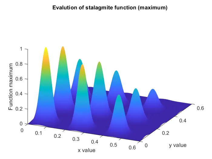
 surface(xx,yy,-f)
 xlabel('x value')
 ylabel('y value')
 zlabel('Function maximum')
 shading interp
 [inputs,fval]=ga(@stalagmite,2)

Clear all (to clear all the stored data to a variable, close all (to close all Matlab fig. window),clc (to clear the command window) commands are used.

2D mesh is created using meshgrid command from x and y vector.(0 t 0 0.6 for 300 values using linspace command)

for loop is created to evaluate the stalagmite function.

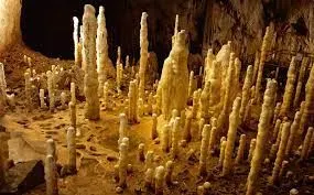
A stalagmite function generally refers to the function with which we are generating values over a stalagmite kind of surface for finding out the local and global maxima and minima of that particularly given function

A stalagmite appears like an inverted stalactite, rising from the floor of a cavern.

xlabel is set as 'x value'

ylabel is set as'y value'

zlabel is set as 'Function maximum')

Creation of the stalagmite function

function[f]=stalagmite(input_vector)

x=input_vector(1);
y=input_vector(2);

f_1x=(sin(5.1*pi*x+0.5))^6;
f_1y=(sin(5.1*pi*y+0.5))^6;

f_2x=exp(-4*log(2)*((x-0.0667)^2)/0.64);
f_2y=exp(-4*log(2)*((y-0.0667)^2)/0.64);

f=-(f_1x*f_1y*f_2x*f_2y);
end

f=function minimum

F=-f =function maximum=-(f_1x*f_1y*f_2x*f_2y)

STEP:II

Optimization of the stalagmite function and finding the global maxima:

clear all
close all
clc

%defining search space
x=linspace(0,0.6,300);
y=linspace(0,0.6,300);

%creating a 2D mesh

[xx yy]=meshgrid(x,y);

% evaluating stalagmite function
 for i=1:length(xx)
   for  j=1:length(yy)
     input_vector(1)=xx(i,j);
     input_vector(2)=yy(i,j);
     f(i,j)=stalagmite(input_vector);
     end
 end
 surface(xx,yy,-f)
 xlabel('x value')
 ylabel('y value')
 zlabel('Function maximum')
 shading interp
 [inputs,fval]=ga(@stalagmite,2)


%study 1
 num_cases=50;

tic
%study 1 statistical behaviour
for i=1:num_cases
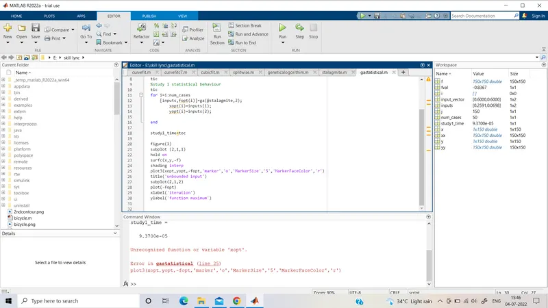
    [inputs,fopt(i)]=ga(@stalagmite,2);
        xopt(i)=inputs(1);
        yopt(i)=inputs(2);
        
end

study1_time=toc
%plotting the graph

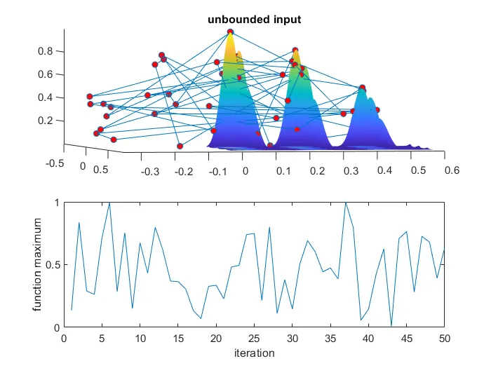
figure(1)
subplot (2,1,1)
hold on
surfc(x,y,-f);
shading interp
plot3(xopt,yopt,-fopt,'marker','o','markersize',5,'markerfaceColor','r');
title('unbounded input')
subplot(2,1,2)
plot(-fopt);
xlabel('iteration')
ylabel('function maximum')


%study 2
num_cases=50;

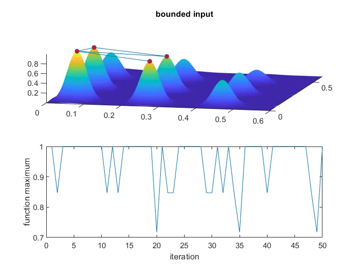
%study 2 statistical behaviour(bounded)
tic
for j=1:num_cases
    [inputs,fopt(j)]=ga(@stalagmite,2,[],[],[],[],[0;0],[0.6;0.6]);
        xopt(j)=inputs(1);
        yopt(j)=inputs(2);
        
end

study2_time=toc

%plotting the graph
figure(2)
subplot (2,1,1)
hold on
surfc(x,y,-f);
shading interp
plot3(xopt,yopt,-fopt,'marker','o','markersize',5,'markerfaceColor','r');
title('bounded input')
subplot(2,1,2)
plot(-fopt);
xlabel('iteration')
ylabel('function maximum')


%study 3
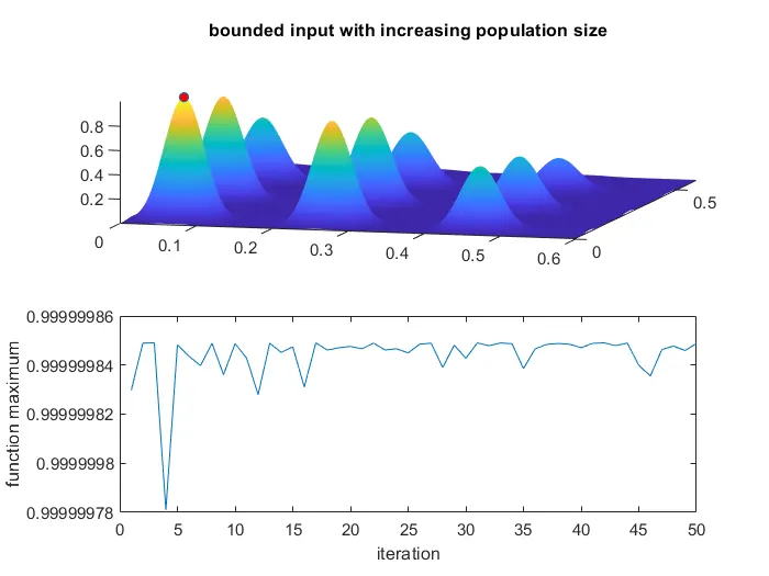
options=optimoptions('ga','populationsize',400)

tic
%study 3 statistical behaviour(increasing population size)
for k=1:num_cases
    [inputs,fopt(k)]=ga(@stalagmite,2,[],[],[],[],[0;0],[0.6;0.6],[],[],options);
        xopt(k)=inputs(1);
        yopt(k)=inputs(2);
        
end

study3_time=toc

%plotting the graph
figure(3)
subplot (2,1,1)
hold on
surfc(x,y,-f);
shading interp
plot3(xopt,yopt,-fopt,'marker','o','markersize',5,'markerfaceColor','r');
title('bounded input with increasing population size')
subplot(2,1,2)
plot(-fopt);
xlabel('iteration')
ylabel('function maximum')

study3_time=toc
rng("default")

clear all (to clear all the stored data to a variable, close all (to close all Matlab fig. window),clc (to clear the command window) commands are used.

2D mesh is created using mesh grid command from x and y vectors.(0 t 0 0.6 for 300 values using linspace command)

study 1:

statistical behavior (unbounded input)

[inputs,fopt(i)]=ga(@stalagmite,2);

num_cases is taken as 50

plotting using surfc command, optimum values provided,-f is used to find maximum .

tick, tock commands are used to evaluate the time used for optimizing the function.

results: variation in the optimum value of the function.

study 2:

statistical behavior (bounded input)

[inputs,fopt(j)]=ga(@stalagmite,2,[],[],[],[],[0;0],[0.6;0.6];

num_cases is taken as 50

plotting using surfc command, optimum values provided,-f is used to find maximum .

tick, tock commands are used to evaluate the time used for optimizing the function.

results:variation in the optimum value of the function has reduced.

study 3:

statistical behavior (bounded input with increasing population size)

[inputs,fopt(k)]=ga(@stalagmite,2,[],[],[],[],[0;0],[0.6;0.6],[],[],options);

population size:400(increasing the possibilites of finding better optimisation of the fuction.

plotting using surfc command, optimum values provided,-f is used to find maximum .

tick, tock commands are used to evaluate the time used for optimizing the function.

The rng command controls the seed, or starting point, for this value. The "default" values reset it to the original value that MATLAB starts with.

results: variation in the optimum value of the function has reduced to a large extent.

Error:

Resolved:

%study 1 statistical behavior

for i=i:num_cases is replaced by

%study 1 statistical behaviour

for i=1:num_cases

Conclusion: Optimization of the stalagmite function and finding the global maxima of the function is successfully done.

References:

https://www.tutorialspoint.com/genetic_algorithms/genetic_algorithms_quick_guide.htm

https://www.javatpoint.com/genetic-algorithm-in-machine-learning

https://in.mathworks.com/help/gads/ga.html

https://in.mathworks.com/matlabcentral/answers/269639-what-does-command-rng-default-do