Week 9 - FVM Literature Review
Aim:
To describe finite volume methods, differences between finite volume and finite difference methods along with the need for the interpolation schemes in the FVM and flux limiter.
FVM:
The Finite volume method (FVM) is a widely used numerical technique. The fundamental conservation property of the FVM makes it the preferable method in comparison to the other methods, i.e., FEM, and finite difference method (FDM). Also, the FVM’s approach is comparable to the known numerical methods like FEM and FDM, which means that its evaluation of volumes is at discrete places over a meshed geometry.
The FVM transforms the set of partial differential equations into a system of linear algebraic equations. Although the discrete approximation procedure in use in the FVM is distinctive, it also utilizes two basic steps. Firstly, it transforms and integrates the PDEs into balance equations over an element.
The process incorporates the changing of the surface and volume integrals into discrete algebraic relations over elements as well as their surfaces using an integration quadrature of a specified order of accuracy. This will result in a set of semi-discrete equations.
The interpolation profiles are chosen to estimate the variation of the variables within the element and relate the surface values of the variables to their cell values and thus transform the algebraic relations into algebraic equations. In regards to the two steps in the FVM process, your approximation selection affects the overall accuracy of the subsequent numeric.
Difference between FDM and FEM:
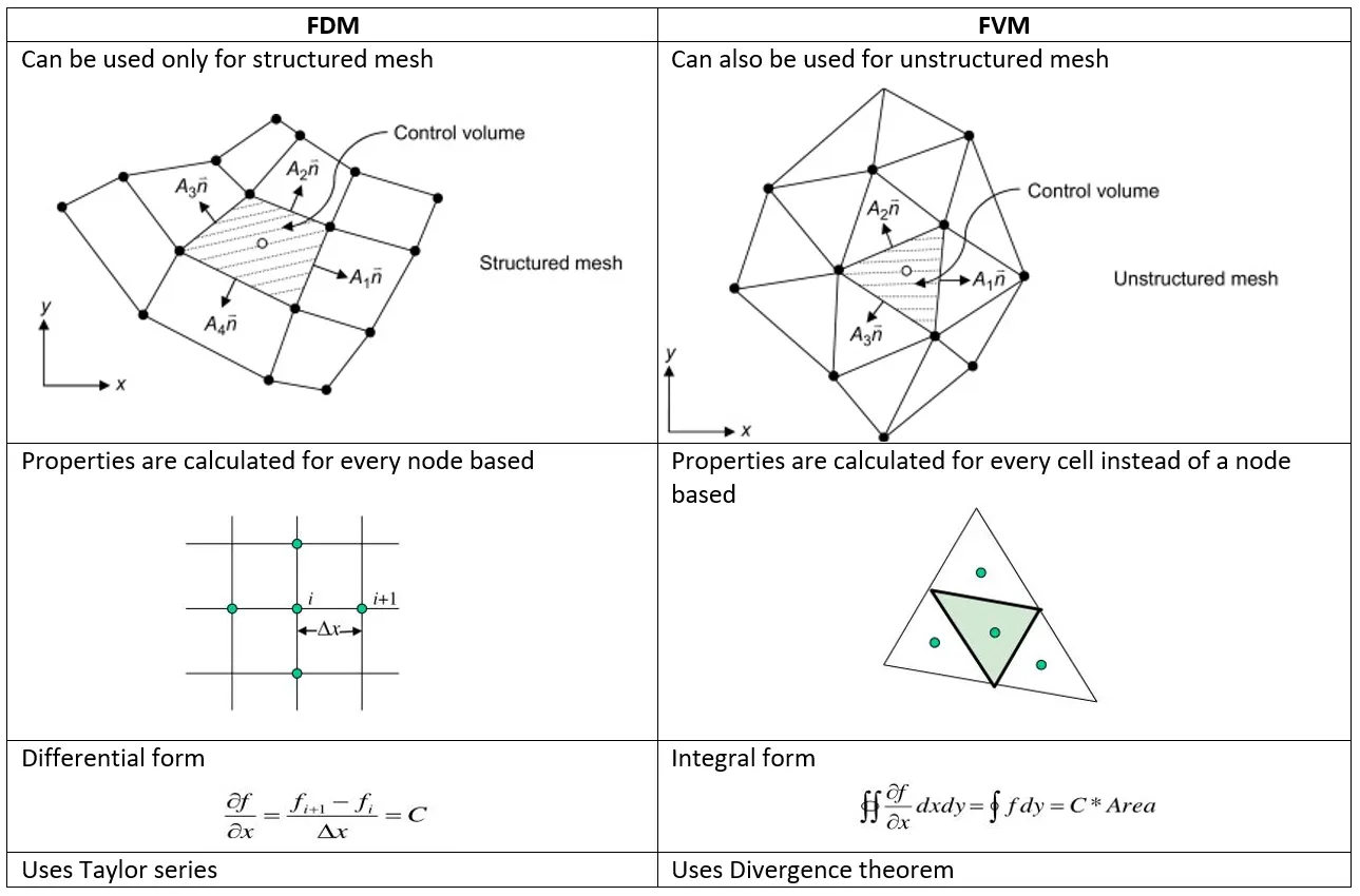
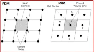
A finite difference method (FDM) discretization is based upon the differential form of the PDE to be solved. Each derivative is replaced with an approximate difference formula (that can generally be derived from a Taylor series expansion). The computational domain is usually divided into hexahedral cells (the grid), and the solution will be obtained at each nodal point.
The FDM is easiest to understand when the physical grid is Cartesian, but through the use of curvilinear transforms the method can be extended to domains that are not easily represented by brick-shaped elements.
The discretization results in a system of equation of the variable at nodal points, and once a solution is found, then we have a discrete representation of the solution.
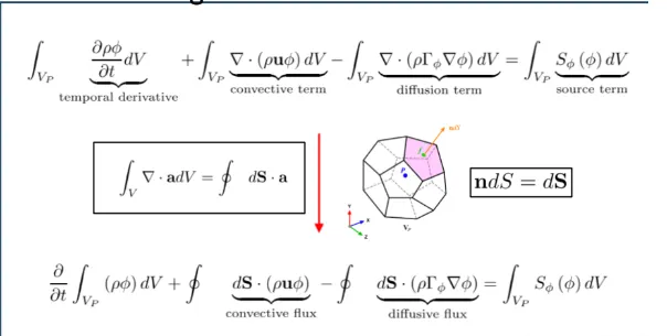
A finite volume method (FVM) discretization is based upon an integral form of the PDE to be solved (e.g. conservation of mass, momentum, or energy).
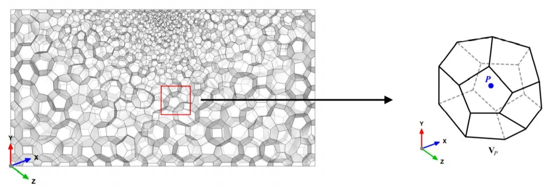
The PDE is written in a form which can be solved for a given finite volume (or cell). The computational domain is discretized into finite volumes and then for every volume the governing equations are solved.
The resulting system of equations usually involves fluxes of the conserved variable, and thus the calculation of fluxes is very important in FVM.
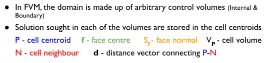
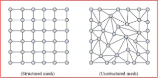
The basic advantage of this method over FDM is it does not require the use of structured grids, and the effort to convert the given mesh in to structured numerical grid internally is completely avoided. As with FDM, the resulting approximate solution is a discrete, but the variables are typically placed at cell centres rather than at nodal points. This is not always true, as there are also face-cantered finite volume methods.
In any case, the values of field variables at non-storage locations (e.g., vertices) are obtained using interpolation.
Gauss Divergence Theorem:
FVM:
FDM:
Grid generation:
The first step in the finite control volume is to discretize the domain into discrete control volumes as shown in figure
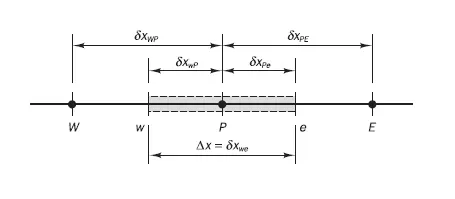
The number of nodal points is placed between A & B. The boundary of the control volume is positioned midway between the two adjacent nodes, thus each node is surrounded by the control volume. The control volume should be set up near the edges of the domain such that the physical boundary and the control volume boundary should coincide with each
other
Discretization
The key step in the finite volume method is to integrate the governing equation over a control volume to yield a discretize equation at its nodal point P. For the control volume
defined above this gives
`int_(Deltav)d/dx(prop**(dT)/dx)**dV+int_(Deltav)SdV=0`
`dV=A**dx``(prop**A**(dT)/dx)_e-(prop**A**(dT)/dx)_omega+SDeltaV=0`
`prop_omega=(propW+propp)/2`
`prop_e=(propE+propp)/2`
Diffusive flux terms are evaluated as
`(prop**A**(dT)/dx)_e=prop_e**A_e**(T_E-T_P)/(deltax_(PE)`
`(prop**A**(dT)/dx)_omega=prop_omega**A_omega**(T_P-T_W)/(deltax_(WP)`
FVM approximates the source trem as
`S**DeltaV=S_u+S_p**T_p`
final equation can be rearranged as
`(prop_e**A_e**(T_E-T_P)/(deltax_(PE)))-(prop_omega**A_omega**(T_P-T_W)/(deltax_(WP)))+(S_u+S_p**T_P)=0`
`((prop_e**A_e)/(deltax_(PW))+(prop_w**A_w)/(deltax_(WP))-S_p)**T_P=((prop_w**A_w)/(deltax_(WP)))**T_W+(prop_e**A_e)/(deltax_(PE))**T_E+S_u`
Interpolation schemes
The approximation of the surface and volume integrals may require values of the variable at locations other than the computational nodes of the control volume (CV). Values at this location are obtained using interpolation formulae.
The interpolation schemes are listed below
First-order upwind scheme:
`u>0`
`u_i-0.5approxu_i-1`
`u_i+0.5approxu_i`
Backward differencing
`I_c=v**(u_i-u_i-1)/dx`
Forward differencing
u<0
`u_i-0.5approxu_i`
`u_i+0.5approxu_i+1`
`I_c=v**(u_i+u_i-1)/dx`
Taylor series expansion
`u(u)_i+0.5=u(u)_i+(vDeltax)/2*((delu)/(delx))_(i+0.5)+(v(Deltax))^2/8*(del^2u)/(delx^2))_(i+0.5)+....`
Central difference approximation
Interpolation polynomial
`p_1(x)=u_Lfrac{x_R-x}{x_R-x_L}+u_Rfrac{x-x_L}{x_R-x_L}`
Average interface values
`u_(i-0.5)approxfrac{u_(i-1)+u_i}{2}, u_(i+0.5)approxfrac{u_i+u_(i+1)}{2}`
`I_c=vfrac{u_(i+1)-u_(i-1)}{2trianglex}`
`u_(i+1)=u_(i+0.5)+frac{trianglex}{2}**(frac{delu}{delx})_(i+0.5)+frac{(trianglex)^2}{8}(frac{del^2u}{delx^2})_(i+0.5)+......`
`u_(i)=u_(i+0.5)-frac{trianglex}{2}**(frac{delu}{delx})_(i+0.5)+frac{(trianglex)^2}{8}(frac{del^2u}{delx^2})_(i+0.5)+......`
`u_(i+0.5)=frac{u_i+u_(i+1)}{2}-frac{(trianglex)^2}{8}*(frac{del^2u}{delx^2})_(i+0.5)`
Quadratic upwind difference scheme (QUICK):
`p_2(x)=u_Lfrac{x-x_M}{x_L-x_M}frac{x_R-x}{x_R-x_L}+u_Mfrac{x-x_L}{x_M-x_L}frac{x_R-x}{x_R-x_M}+u_Rfrac{x-x_L}{x_R-x_L}frac{x-x_M}{x_R-x_M}`
Upwind biased interface values
`u_(i-0.5)approxfrac{3u_i+6u_(i-1)-u_(i-2)}{8}`
`u_(i+0.5)approxfrac{3u_(i+1)+6u_(i)-u_(i-1)}{8}`
`I_c approxvfrac{3u_(i+1)-7u_(i-1)+3u_i+u_(i-2)}{8trianglex}`
`u_(i-0.5)approxfrac{3u_(i-1)+6u_(i)-u_(i+1)}{8}`
`u_(i+0.5)approxfrac{3u_(i)+6u_(i+1)-u_(i+2)}{8}`
`I_c approx-vfrac{3u_(i-1)-7u_(i+1)+3u_i+u_(i+2)}{8trianglex}`
Third order flux approximation.
Second-order overall accuracy (because of the midpoint rule).
Flux limiters:
They are used in high-resolution schemes to avoid spurious oscillations (wiggles) that would otherwise occur with high-order spatial discretization schemes due to shocks, discontinuities, or sharp changes in the solution domain. For smoothly changing solution flux limiters are not used and the spatial derivatives can be implemented with highresolution schemes. If there are discontinuities in the domain the fux limiters change the solution to low and high-resolution schemes depending upon the gradients in the nearby surroundings.
Case-1
Absence of source term in the heat conduction equation
`frac{d}{dx}(K**frac{dT}{dx})=0`
`K*A*(frac{T_E-T_P}{dx})-K*A*(frac{T_P-T_W}{dx)=0`
`frac{2**K**A}{dx}**T_P=frac{K**A}{dx}**T_E+frac{K*A}{dx}**T_W`
`frac{2**K**A}{dx}**T_P=frac{K**A}{dx}**T_A+frac{K*A}{dx}**T_E`
`frac{2**K**A}{dx}**T_P=frac{K**A}{dx}**T_B+frac{K*A}{dx}**T_W`
Case-2
Presence of source term in the heat conduction equation
`frac{d}{dx}(K**frac{dT}{dx})+q=0`
`frac{2**K**A}{dx}**T_P=frac{K**A}{dx}**T_E+frac{K*A}{dx}**T_W+q**A**dx`
`frac{2**K**A}{dx}**T_P=frac{K**A}{dx}**T_A+frac{K*A}{dx}**T_E+q**A**dx`
`frac{2**K**A}{dx}**T_P=frac{K**A}{dx}**T_B+frac{K*A}{dx}**T_W+q**A**dx`