Week 4.1 - Genetic Algorithm

AIM: To find global maxima of the stalagmite function using MATLAB.

THEORY: Optimization describes a class of problems for finding the input to a given function that results in the minimum or maximum output from the function. Optimization is the process of selection from the set of values for the imposed targets and the constraints and the optimization is a kind of decision-making process. Productivity, strength, reliability, efficiency, utilization these all are the maximizing factor of optimization. It is very difficult to manage and select the appropriate range of values for the defined targets and constraints. This process is mainly used to find the best results.

POPULATION ALGORITHM: This algorithm is mainly used to maintains an entire set of candidate solutions, and each of the solutions corresponding to a unique point in the search space of the problem known as population algorithm.

SOME OF THE POPULATION BASED ALGORITHMS:

• Genetic algorithm
• Differential evolution
• Particle swarm optimization

GENETIC ALGORITHM(GA): Genetic algorithm is nothing it is a method for solving both constraints and unconstrainted optimization problems that is based on natural selection the process that drives biological evolution. The genetic algorithm repeatedly modifies a population of individual solutions. Genetic algorithm (GA) is a search-based optimization technique based on the principle of genetics and natural selection. It is mainly used to solve optimization problems in research and in machine learning. The genetic algorithm can be Three main components or genetic operators in genetic algorithms are

• Selection
• Crossover
• Mutation

SELECTION: It defined the selection of parents for the next generation using selection function/fitness function which will be the based on the fitness value.

CROSSOVER: Crossover enables the algorithm to extract the best characters from different individuals and recombine them into potentially superior children.

MUTATION: Mutation adds to the diversity of a population and thereby increases the likelihood that the algorithm will generate individuals with better fitness values.

OUTLINE OF THE GENETIC ALGORITHM WORKS:

1. The algorithm is creating a random initial population
2. The algorithm creates a sequence of new populations. The algorithm uses the individuals in the current generation to create the next population. Below the following steps uses to create the new population.

• Raw fitness scores is nothing but the scores each member of the current population by computing its fitness value the fitness value is called raw fitness scores.
• The Raw fitness scores to convert into a more usable range of values. This is called expectation values.
• The best fitness values based on their select members, called parents.
• The children will produce from the parents. These childrens are produced either by making random changes to a single parent – mutation by combining the pair of parents- crossover.
• It will replace the current population with the children to form the next generation.
• When the current population is replaces the children to form the next generation.
• This process repeats itself until it gets converged to a optimal value.

STALAGMITE FUNCTION:

were,

f (x, y) = f1, xf2, xf1, yf2, y

f1, x = [sin (5.1πx + 0.5)] ^6

f1, y = [sin (5.1πy + 0.5)] ^6

f2, x = exp [ − 4 ln (2) ((x − 0.0667) ^2/ 0.64))]

f2, y = exp [ − 4 ln (2) ((y − 0.0667) ^ 2/ 0.64))]

OBJECTIVE:

To optimize the stalagmite function and to find the global maxima of the function.

Stalagmite function program:

% Genetic Algorithm Function Code.
function [P] = gene_alg(input_vector) 
x = input_vector(1);
y = input_vector(2);

f1x = (sin(5.1*pi*x + 0.5)).^6;
f1y = (sin(5.1*pi*y + 0.5)).^6;

t1  = ((x-0.0667).^2/(0.64));
t2  = ((y-0.0667).^2/(0.64));

f2x = exp(-4.*log(2)*t1);
f2y = exp(-4.*log(2)*t2);

P = -(f1x.*f2x.*f1y.*f2y);

end

Study 1 : The first study denotes with the unbounded inputs provided for calculating the value of global maxima this is the first step of study for this function

MAIN PROGRAM PART 1 :

% Stalagmite - Genetic Algorithm Concept
clear all
close all
clc

% Search space for the function.
x = linspace(0,1,300);
y = linspace(0,1,300);

% Use of meshgrid command to get 2D arrays.
[xx yy] = meshgrid(x,y);

% Number of iterations performed by the function.
num_case = 150

% Surface plot for genetic algorithm function.
  for i = 1:length(xx)
      for j = 1:length(yy);
          input_vector(1) = xx(i,j);
          input_vector(2) = yy(i,j);
          p(i,j) = gene_alg(input_vector);
      end
  end

% Generate the surface for the plot
surfc(xx,yy,-p);

% Remove the line produce by meshgrid
shading interp

% Initiate timer for calculating survey time
tic
  for i = 1:num_case
      % Calculate the optimized value of the function
      [inputs,popt(i)] = ga(@gene_alg,2);
      % Optimised value at ech iterations.
      xopt(i) = inputs(1);
      yopt(i) = inputs(2);
  end

% Display time taken to complete the survey
survey1_time = toc

% Plot the graph with the obtained optimized data
figure(1)
subplot(2,1,1)
surfc(xx,yy,-p);
hold on 
shading interp
plot3(xopt,yopt,-popt,'Marker','o','MarkerSize',5,'MarkerFaceColor','g');
title('Unbounded Inputs');
xlabel('x value ');
ylabel('y value ');
grid on
subplot(2,1,2)
plot(-popt);
xlabel('iterations');
ylabel('function with min value');
 

STUDY 2 : This second study denotes with the bounded inputs provided for calculating the value of global maxima.

Main program part 2:

% Initiate timer for calculating survey time
tic
  for j = 1:num_case
       % Calculate the optimized value of the function
      [inputs,popt(j)] = ga(@gene_alg,2,[],[],[],[],[0;0],[1;1]);
       % Optimised value at ech iterations
      xopt(j) = inputs(1);
      yopt(j) = inputs(2);
  end

 % Display time taken to complete the survey
 survey2_time = toc

% Plot the graph with the obtained optimized data
figure(2)
subplot(2,1,1)
surfc(xx,yy,-p);
hold on 
shading interp
plot3(xopt,yopt,-popt,'Marker','o','MarkerSize',5,'MarkerFaceColor','g');
title('Bounded Inputs');
xlabel('x value ');
ylabel('y value');
grid on
subplot(2,1,2)
plot(-popt);
xlabel('iterations');
ylabel('function with min value');
 

Study 3: This third study denotes with the bounded inputs with a varied population size for best optimization to calculate the value of globa maxima.

Main program part 3:

%Increase the population by using the 'optimoption' command
options = optimoptions('ga','PopulationSize',300)

% Initiate timer for calculating survey time
tic
  for k = 1:num_case
      % Calculate the optimized value of the function.
      [inputs,popt(k)] = ga(@gene_alg,2,[],[],[],[],[0;0],[1;1],[],[],options);
        % Optimised value at ech iterations.
      xopt(k) = inputs(1);
      yopt(k) = inputs(2);
  end

  % Display time taken to complete the survey
  survey3_time = toc

% Plot the graph with the obtained optimized data
figure(3)
subplot(2,1,1)
surfc(xx,yy,-p);
hold on 
shading interp
plot3(xopt,yopt,-popt,'Marker','o','MarkerSize',5,'MarkerFaceColor','g');
title('Statistical study with increase in population');
xlabel('x value');
ylabel('y value ');
grid on
subplot(2,1,2)
plot(-popt);
xlabel('iterations');
ylabel('function with min value');

Explanation of the above program:

• The stalagmite function was mentioned with appropriate argument vectors.
• The program has been divided into three part of the studies based on the limitations of the previous study.
• First part of the study denotes with unbounded inputs, thereby expanding the boundary wherein the results can be obtained.
• Second part of the study denotes with bounded inputs providing a better solution for the drawback faced.
• The Third part of the study denotes with lays a appreciable platform to determine the exact solution. Plots of all the three studies have been displayed, thus giving a clear result.

RESULTS

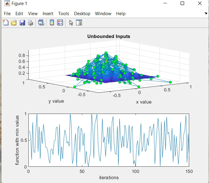
This image denotes the results for the unbounded inputs. thus the image providing idea of the global maxima but its only denote maximum lies between the intevals so we can show for bounded inputs also that can give a more best results.

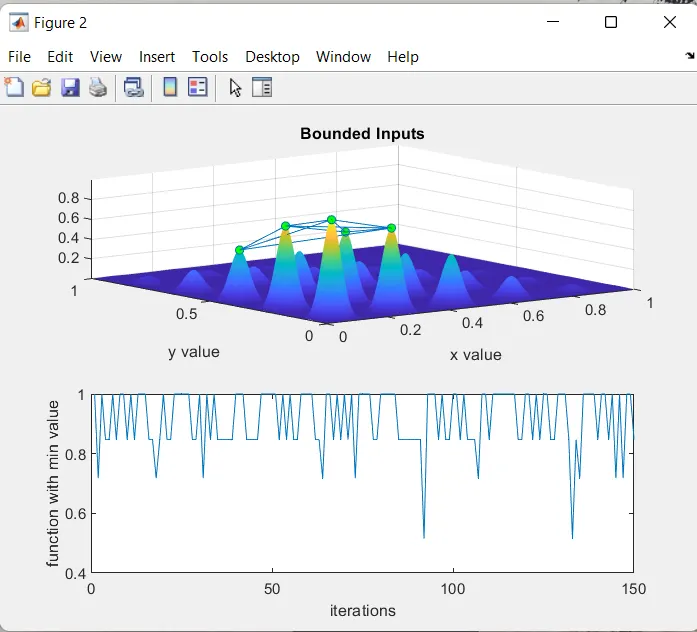
This image represents the value of bounded inputs global maxima so we can specify a population size that can justify the results and it can provide the correct solution.

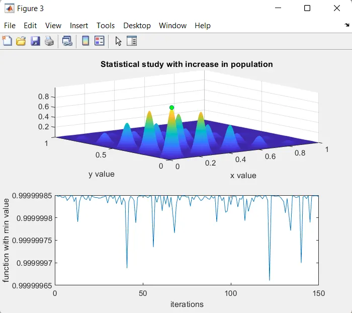
This image denotes the use of population method within the bounded inputs increase the exact value of the global maxima. This image assumed the value of population size.

GLOBAL MAXIMA out comes:

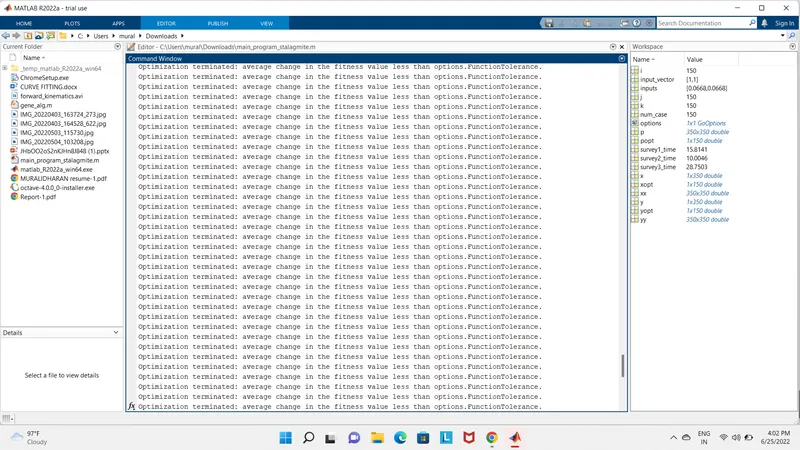
workspace denotes the value of inputs and outputs of the given program.