Week 3 - Solving second order ODEs
CURVE FITTING
OBJECTIVE:
In this challenge I have to write code to fit a linear and cubic polynomial for the Cp data and also create a plot linear, cubic curves with axis along with the raw data points and then I create a code to split wise method. Finally, I will explain the parameters used to measure the fitness characteristics for both the curves.
THEORY:
Curve fitting is nothing but the process of constructing a curve or mathematical function that has the best fit to a series of the data points and it is possibly to subject to constraints. Curve fitting is one of the most powerful and most widely used analysis tools in origin.
Curve fitting relationship between dependent variables it is depends on other variable and the independent variable is depending on no other variable. For example, linear polynomial
Y = aX +b
Were,
Y = specific heat (‘dependent variable since it is depending on temperature’)
X = temperature (‘independent variable’)
a & b = coefficients
In the curve fitting we have to consider the experimental data (x&y) here, x = temperature, y = specific heat (Cp) plotting the experimental data gives the data curve as shown.
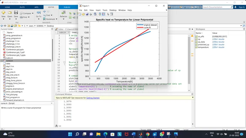
Linear polynomial fitting: curve fitting is done by using linear polynomial equation (having degree one)
Y = aX +b
It forms the linear fitting only and suitable for only linear data.
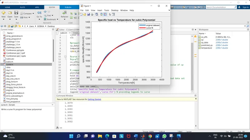
Cubic polynomial fitting: curve fitting is done by using cubic polynomial equation (having degree three)
ax^2 + bx^2 + cx + d = 0
It forms the cubic fitting and suitable for non-linear data.
Curve fitting approach:
Calculation of coefficients: the command of ‘profit’ helps to find the coefficient of the polynomial equation for the given degree.
Finding the predicted values:
The command of ‘polyval’ helps to find the evaluate the predicted ‘y’ values.
Split wise method:
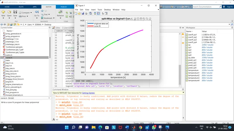
Split wise method is nothing but depending on the trend of the data we can split it accordingly and then program curve fitting process for each segment separately.
Split wise method is used to reduce the constraints in the fitting process and the result will in better curve.
The program for cubic polynomial:
% Write a curve fit program for cubic polynomial
clear all
close all
clc

%preparing the data
cp_data=load('data');
temparature=cp_data(:,1)         % First column is temperature data
cp=cp_data(:,2)                  % second column is cp data

%curve fit
%cp=a*T^2+b*T+c
co_effs=polyfit(temparature,cp,3); % the polyfit command to estimate coefficient a,b
predicted_cp=polyval(co_effs,temparature); % polyval command to calculate predicted value of cp

% compare my curve fit with the original data
plot(temparature,cp,'linewidth',3) % plotting curve for original data set
hold on
plot(temparature,predicted_cp,'linewidth',3,'color','r') % plotting curve for predicted data set
xlabel('Temparature[K]')           % assuming the name of xlabel
ylabel('specific Heat[KJ/Kmol-K]') % assuming the name of ylabel
axis([0 4000 900 1400]);
title('Specific heat vs Temperature for Linear Polynomial')
legend('original dataset','curve fit') % providing legends to curve
This image for cubic polynomial curve fitting:
This program for linear polynomial:
% Write a curve fit program for linear polynomial
clear all
close all
clc
%preparing the data
cp_data=load('data');
temparature=cp_data(:,1) % First column is temperature data
cp=cp_data(:,2) % second column is cp_data
%curve fit
%cp=a*T^2+b*T+c
co_effs=polyfit(temparature,cp,1); % the polyfit command to estimate coefficient a,b
predicted_cp=polyval(co_effs,temparature); % polyval command to calculate predicted value of cp
% compare my curve fit with the original data
plot(temparature,cp,'linewidth',3) % plotting curve for original data set
hold on
plot(temparature,predicted_cp,'linewidth',3,'color','r') % plotting curve for predicted data set
xlabel('Temparature[K]') % assuming the name of xlabel
ylabel('specific Heat[KJ/Kmol-K]') % assuming the name of ylabel
axis([0 4000 900 1400]);
title('Specific heat vs Temperature for Linear Polynomial')
legend('original dataset','curve fit') % providing legends to curveThis image for linear polynomial curve fitting:
This program for split-wise curve fitting:
% spilt - wise curve fits
clear all
close all
clc

%preparing the data.
cp_data=load('data');
temperature=cp_data(:,1)
cp=cp_data(:,2)

%spitting data.
temperature1=cp_data(1:800,1);
cp1= cp_data(1:800,2);

temperature2=cp_data(801:1600,1);
cp2= cp_data(801:1600,2);

temperature3=cp_data(1601:2400,1);
cp3= cp_data(1601:2400,2);


temperature4=cp_data(2401:3200,1);
cp4= cp_data(2401:3200,2);

%considering cubic polynomial; y =aX^3+bX^2+cX+d.

coeiff_cp1= polyfit(temperature1,cp1,3);
predi_cp1=polyval(coeiff_cp1,temperature1);

coeiff_cp2= polyfit(temperature2,cp2,3);
predi_cp2=polyval(coeiff_cp2,temperature2);

coeiff_cp3= polyfit(temperature3,cp3,3);
predi_cp3=polyval(coeiff_cp3,temperature3);

coeiff_cp4= polyfit(temperature4,cp4,3);
predi_cp4=polyval(coeiff_cp4,temperature4);

% plotting Results.
plot(temperature, cp, 'Linewidth', 3);
hold on
plot(temperature1,predi_cp1,'Linewidth', 3,'color', 'r');
hold on
plot(temperature2,predi_cp2,'Linewidth',3,'color', 'g');
hold on
plot(temperature3,predi_cp3,'Linewidth',3,'color', 'b');
hold on
plot(temperature4,predi_cp4,'Linewidth',3,'color','m');
hold on
xlabel('temperature [k] ');
ylabel('specific Heat [k]/kmo1-k]');
axis([0  4000 900 1400]);
title('split-Wise vs Orginal1 Curve Fit');
legend('origional data set', 'curve fit', 'Location', 'northwest');
This image for split-wise curve fitting:
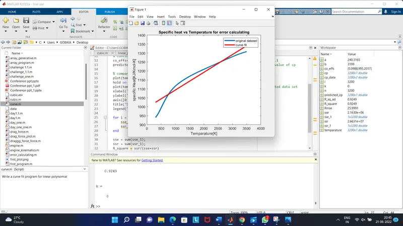
This program for error calculating in curve fitting:
% Write a curve fit program for error calculating
clear all
close all
clc

% loading the data to matlab
cp_data=load('data');
temparature=cp_data(:,1)         % First column is temperature data
cp=cp_data(:,2)                  % second column is cp data

% considering first order polynomial ; Y = aX+b
co_effs=polyfit(temparature,cp,1); % the polyfit command to estimate coefficient a,b.1
predicted_cp=polyval(co_effs,temparature); % polyval command to calculate predicted value of cp

% compare my curve fit with the original data
plot(temparature,cp,'linewidth',3) % plotting curve for original data set
hold on
plot(temparature,predicted_cp,'linewidth',3,'color','r') % plotting curve for predicted data set
xlabel('Temparature[K]')           % assuming the name of xlabel
ylabel('specific Heat[KJ/Kmol-K]') % assuming the name of ylabel
axis([0 4000 900 1400]);
title('Specific heat vs Temperature for Linear Polynomial')
legend('original dataset','curve fit') % providing legends to curve

for i = 1:length(cp_data)
    sse_1(i)= (predicted_cp(i)-cp(i))^2;
    ssr_1(i)= (predicted_cp(i)-mean(cp))^2;
end

sse = sum(sse_1);
ssr = sum(ssr_1);
R_square = ssr/(sse+ssr)
k = 0
n = length(cp_data);
a = (1-R_square)*(n-1);
b = (n-k-1);
R_sq_ad = (1-a/b);
Rmse = (sse/n)^0.5;
This image for error calculating curve fitting:
Conclusion:
Finally, I wrote a program code for curve fitting and I plotted curves for linear, cubic polynomial equations, split wise method also and I successfully explained the parameters used to measure the fitness characteristics for all the curves.