Week 9 - FVM Literature Review

Finite Volume Method

• The finite volume method (FVM) is a method for representing and evaluating partial differential equations in the form of algebraic equations.
• Finite volume refers to the small volume surrounding each node point on a mesh means the grid points where variables are stored are typically defined as being at the centre of each control volume.
• The method starts by dividing the flow domain into a number of small control volumes.
• In the finite volume method, volume integrals in a partial differential equation that contain a divergence term are converted to surface integrals, using the divergence theorem. These terms are then evaluated as fluxes at the surfaces of each finite volume.
• Because the flux entering a given volume is identical to that leaving the adjacent volume, these methods are conservative.
• Similar to the finite difference method (FDM) or finite element method (FEM), values are calculated at discrete places on a meshed geometry.
• Since they are based on applying conservation principles over each small control volume, global conservation is also ensured.
• The advantage of the finite volume method is that it is easily formulated to allow for unstructured meshes, and this method is used in many computational fluid dynamic packages.

In finite difference method:

• The grid is linear and aligned so that all grid points lie in a straight line .
• Main thing is that the properties are considered to concentrated at a single point.

In finite volume method:

• The method is applied over a volume such that the governing equation is valid over the entire volume .
• The properties are assumed to be concentrated at the geometric centre of the volume concerned.

Interpolation schemes in Finite Volume Method:

Interpolation is a process to estimate the values at unknown points by using the points with known value and sample points on either sides of the unknown point. In FVM, interpolation schemes are used to find values of volume integrals required at the points other than nodes.

The different interpolation schemes are:

1. Upwind Interpolation Scheme (UDS)

2. Linear Interpolation Scheme

3. Quadratic Upwind Interpolation Scheme

4. Hybrid Interpolation Scheme

5. Total variation Diminishing Scheme

6. Essentially Non-oscillatory interpolation Scheme

In the finite volume formulation, evaluation of surface and volume integrals sometimes requires the values of unknown variables at locations other than the computational nodes of the control volume. These values are obtained by employing certain interpolation schemes.

FLUX LIMITERS:

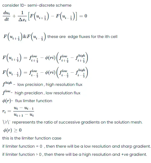
For convective fluid flow, it is observed that the low order schemes are usually stable but quite dissipative in nature around the points of discontinuity or shocks while the higher order schemes are unstable in nature and show oscillations in the vicinity of discontinuity or shocks. Highly accurate and oscillation free schemes are known as High Resolution Schemes.

Flux Limiter functions are used to fine tune the higher order and lower order schemes in such a way that the resulting scheme gives a higher order accuracy in the smooth region of the flow and maintains first order accuracy in the vicinity of shocks and discontinuities. For such a scheme TVD scheme is employed.

The flux limiter function is constrained to be greater than or equal to zero. It assumes a value of 0 near discontinuities and a value of 1 away from them. Hence it switches between higher order scheme and lower order scheme for numerical representation of flux, thereby keeping the scheme stable and accurate throughout.

Note that flux limiters are also referred to as slope limiters because they both have the same mathematical form, and both have the effect of limiting the solution gradient near shocks or discontinuities. In general, the term flux limiter is used when the limiter acts on system fluxes and slope limiter is used when the limiter acts on system states (like pressure, velocity etc.).