Week 7 - Simulation of a 1D Super-sonic nozzle flow simulation using Macormack Method
Aim:
- To simulate the isentropic flow through a quasi 1D subsonic-supersonic nozzle.
- To derive both the conservation and non-conservation forms of the governing equations and sovle them using the MacCormack's technique.
Problem statement :
- To determine the steady-state temperature distribution for the flow-field variables and to investigate the difference between the two forms of governing equations by comparing their solutions.
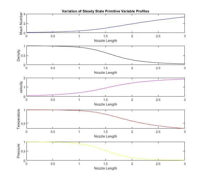
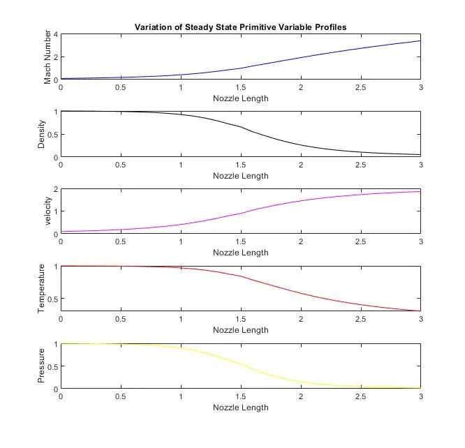
- To plot steady-state distribution of primitive variables inside the nozzle.
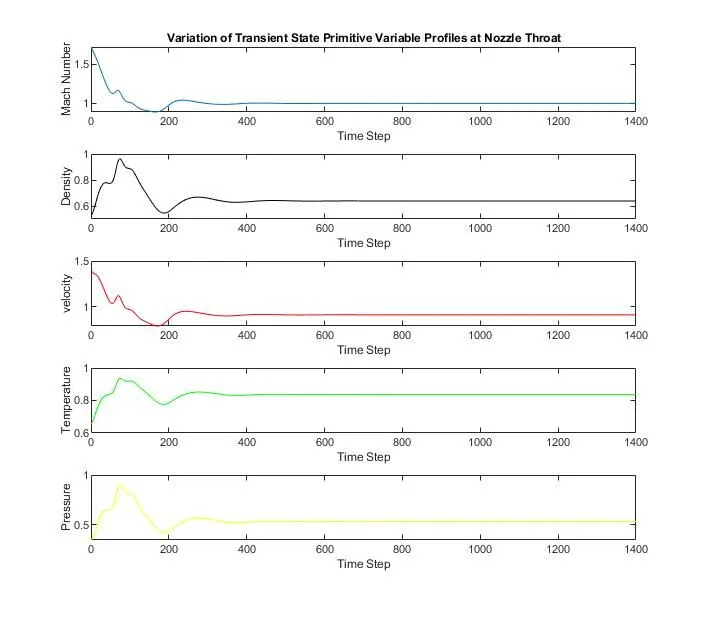
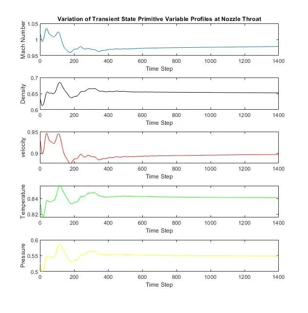
- To plot time-wise variation of the primitive variables.
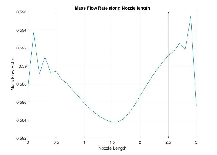
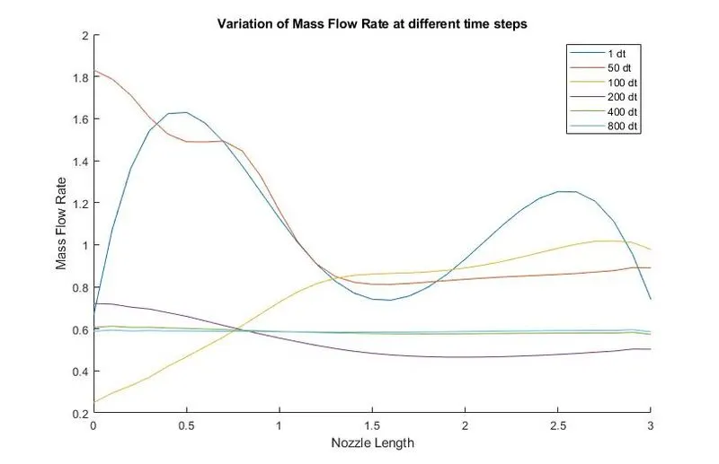
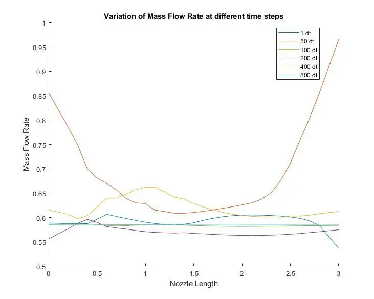
- To plot variation of Mass flow rate distribution inside the nozzle at different time steps during the time-marching process.
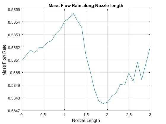
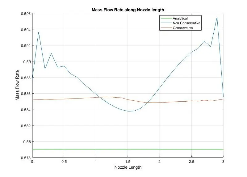
- To plot comparison of Normalized mass flow rate distributions of both forms.
Nozzle diagram :
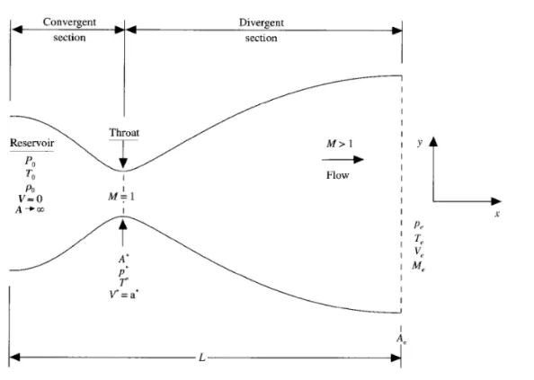
- At convergent section the flow velocity is less than the sound velocity therefore there mach number is less than 1.
- At throat section the flow velocity is equal to the sound velocity therefore there mach number is equal to 1.
- At divergent section the flow velocity is greater than the sound velocity therefore there mach number is greater than 1.
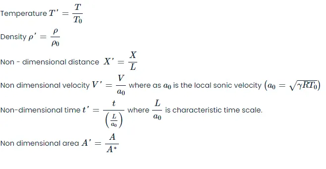
Non Dimensional Quantities :
Also as part of the problem setup we represent quantities in terms of non-dimensional quantities
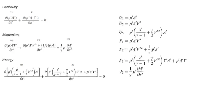
Non Conservative form :
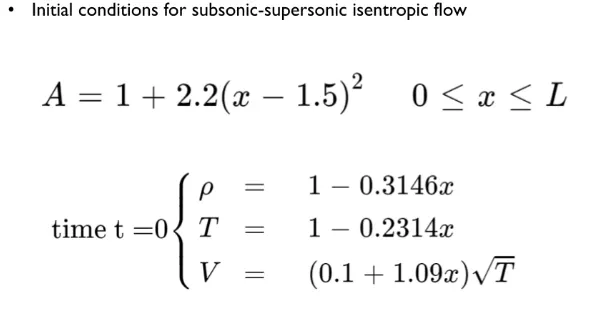
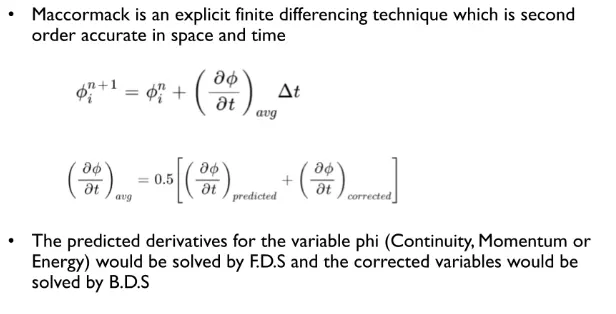
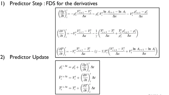
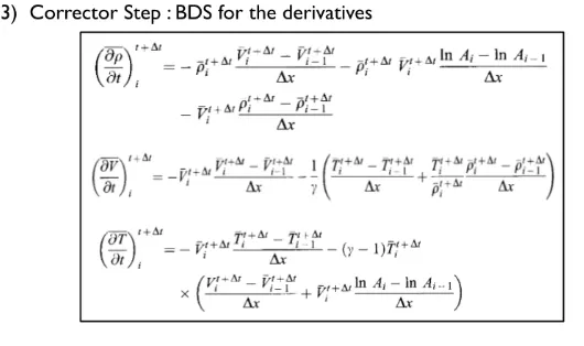
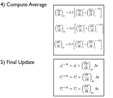
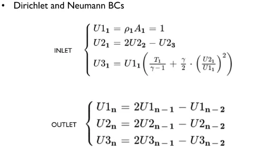
Boundary conditions :
In our case, we are having a subsonic flow in the convergent section (M<1), choked flow at the throat section (M=1) and supersonic outflow in the divergent section (M>1). So by using method of characteristics for an unsteady, one-dimensional flow we can precisely allot inflow and outflow boundary conditions and can identify which quantities to state at the boundaries.
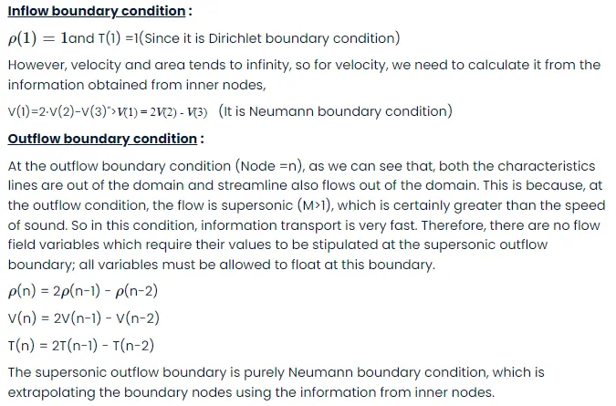
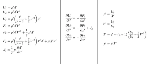
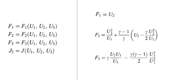
Conservative form :
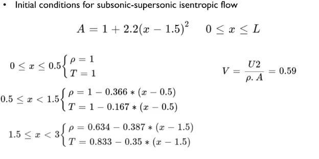
In conservative form, we will initialize the nozzle profile rationally. As in conservative form, seen above from the governing equations, we have solution vectors, flux terms and a source term. So it is the prior matter of concern to state initial and boundary conditions in those terms rather than that of primitive variables.
clc
clear all
close all

% Inputs
n =31;
l = 3;
x = linspace(0,l,n);
dx = x(2)-x(1);
gamma = 1.4;

% Initial Profiles
rho = 1-0.3146*x;
T = 1-0.2314*x;
v = (0.1+1.09*x).*T.^0.5;
A = 1+2.2*(x-1.5).^2;

% Time Step
nt = 1400;
CFL = 0.5;

th = round(n/2);

% Time Loop
for i = 1:nt

    dt(i) = min((CFL*dx)./(v+sqrt(T)));

    rho_old = rho;
    T_old = T;
    v_old = v;

    % Predictive Method
    for j = 2:n-1

        dvdx = (v(j+1)-v(j))/dx;
        dlogA_dx = (log(A(j+1))-log(A(j)))/dx;
        drhodx  = (rho(j+1)-rho(j))/dx;
        dTdx = (T(j+1)-T(j))/dx;

        %Prdictive step

        % Continuity Equation
        drhodt_p(j) = -rho(j)*dvdx-rho(j)*v(j)*dlogA_dx-v(j)*drhodx;

        % Momentum Equation
        dvdt_p(j) = -v(j)*dvdx-(1/gamma)*(dTdx+(T(j)/rho(j))*drhodx);

        % Energy Equation
        dTdt_p(j) = -v(j)*dTdx-(gamma-1)*T(j)*(dvdx+v(j)*dlogA_dx);

        %Predictive Solution update
        rho(j) = rho_old(j) + drhodt_p(j)*dt(i);
        v(j) = v_old(j) + dvdt_p(j)*dt(i);
        T(j) = T_old(j) + dTdt_p(j)*dt(i);
    end

    % Corrective Method

    for j = 2:n-1

        dvdx = (v(j)-v(j-1))/dx;
        dlogA_dx = (log(A(j))-log(A(j-1)))/dx;
        drhodx  = (rho(j)-rho(j-1))/dx;
        dTdx = (T(j)-T(j-1))/dx;

        %Prdictive step

        % Continuity Equation
        drhodt_c(j) = -rho(j)*dvdx-rho(j)*v(j)*dlogA_dx-v(j)*drhodx;

        % Momentum Equation
        dvdt_c(j) = -v(j)*dvdx-(1/gamma)*(dTdx+(T(j)/rho(j))*drhodx);

        % Energy Equation
        dTdt_c(j) = -v(j)*dTdx-(gamma-1)*T(j)*(dvdx+v(j)*dlogA_dx);

        end

    % Average Values

    drhodt = 0.5*(drhodt_p+drhodt_c);
    dvdt = 0.5*(dvdt_p+dvdt_c);
    dTdt = 0.5*(dTdt_p+dTdt_c);

    % Final Solution
    for k = 2:n-1

        rho(k) = rho_old(k) + drhodt(k)*dt(i);
        v(k) = v_old(k) + dvdt(k)*dt(i);
        T(k) = T_old(k) + dTdt(k)*dt(i);
    end

    % BCs
    % Inlet

    rho(1) = 1;
    T(1) = 1;
    v(1) = 2*v(2)-v(3);

    %Outlet
    v(n) = 2*v(n-1)-v(n-2);
    rho(n) = 2*rho(n-1)-rho(n-2);
    T(n) = 2*T(n-1)-T(n-2);

    % Pressure
    p = rho.*T;

    % Mach Number
    M = v./sqrt(T);

    % Mass Flow Rate
    m = rho.*A.*v;

    % Primitive Variables at throat
    M_throat(i) = M(th);
    rho_throat(i) = rho(th);
    v_throat(i) = v(th);
    T_throat(i) = T(th);
    p_throat(i) = p(th);

    % Mass flow rate at different time steps
    figure(4)
    hold on
    if i ==1
        plot(x,m)
    end
    if i ==50
        plot(x,m)
    end
    if i ==100
        plot(x,m)
    end
    if i ==200
        plot(x,m)
    end
    if i ==400
        plot(x,m)
    end
    if i ==800
        plot(x,m)
    end

end

% Plotting

% Mass flow rate at different time steps
xlabel('Nozzle Length')
ylabel('Mass Flow Rate')
legend('1 dt','50 dt','100 dt','200 dt','400 dt','800 dt')
title('Variation of Mass Flow Rate at different time steps')
% Steady State Primitive Variable Profiles

figure(1)
subplot(5,1,1)
plot(x,M,'b')
xlabel('Nozzle Length')
ylabel('Mach Number')
title('Variation of Steady State Primitive Variable Profiles')
subplot(5,1,2)
plot(x,rho,'k')
xlabel('Nozzle Length')
ylabel('Density')
subplot(5,1,3)
plot(x,v,'m')
xlabel('Nozzle Length')
ylabel('velocity')
subplot(5,1,4)
plot(x,T,'r')
xlabel('Nozzle Length')
ylabel('Temperature')
subplot(5,1,5)
plot(x,p,'y')
xlabel('Nozzle Length')
ylabel('Pressure')

% Transient State Primitive Variable Profiles
figure(2)
subplot(5,1,1)
plot(M_throat)
xlabel('Time Step')
ylabel('Mach Number')
title('Variation of Transient State Primitive Variable Profiles at Nozzle Throat')
subplot(5,1,2)
plot(rho_throat,'k')
xlabel('Time Step')
ylabel('Density')
subplot(5,1,3)
plot(v_throat,'r')
xlabel('Time Step')
ylabel('velocity')
subplot(5,1,4)
plot(T_throat,'g')
xlabel('Time Step')
ylabel('Temperature')
subplot(5,1,5)
plot(p_throat,'y')
xlabel('Time Step')
ylabel('Pressure')

% Mass Flow rate
figure(3)
plot(x,m)
xlabel('Nozzle Length')
ylabel('Mass Flow Rate')
title('Mass Flow Rate along Nozzle length')
grid on
clc
clear all
close all

% Inputs
n =31;
x = linspace(0,3,n);
dx = x(2)-x(1);

th = round(n/2);

for i = 1:length(x)
if x(i) <= 0.5
    rho(i) = 1;
    T(i) = 1;
end
end

for i = 1:length(x)
if x(i)>0.5 && x(i)<1.5
    rho(i) = 1-0.366*(x(i)-0.5);
    T(i) = 1-0.167*(x(i)-0.5);
end
end

for i = 1:length(x)
if x(i) >= 1.5
    rho(i) = 0.634-0.3879*(x(i)-1.5);
    T(i) = 0.833-0.3507*(x(i)-1.5);
end
end

% Initial Profiles
A = 1+ 2.2*(x-1.5).^2;
v = 0.59./(rho.*A);

gamma = 1.4;

% Time Step
nt = 1400;
CFL = 0.5;

dt = min((CFL*dx)./(v+sqrt(T)));

U1=rho.*A;
U2=rho.*A.*v;
U3=rho.*((T./(gamma-1))+(gamma/2).*v.^2).*A;


% Time Loop
for i = 1:nt


    U1_old = U1;
    U2_old = U2;
    U3_old = U3;

    F1=U2;
    F2=((U2.^2)./U1)+((gamma-1)/gamma)*(U3-(gamma/2)*(((U2).^2)./U1));
    F3=(((gamma)*(U2.*U3))./U1)-(((gamma*(gamma-1))/2)*((U2.^3)./U1.^2));

    % Predictive Method
    for j = 2:n-1


       dU1dt_p(j) = -(F1(j+1)-F1(j))/dx;

       J2 = (1/gamma)*rho(j)*T(j)*(A(j+1)-A(j))/dx;

       dU2dt_p(j) = -(F2(j+1)-F2(j))/dx + J2;

       dU3dt_p(j) = -(F3(j+1)-F3(j))/dx;

        %Predictive Solution update
        U1(j) = U1(j) + dU1dt_p(j)*dt;
        U2(j) = U2(j) + dU2dt_p(j)*dt;
        U3(j) = U3(j) + dU3dt_p(j)*dt;

    end

    %Update F & Pritimitive variables vector for J2
    rho = U1./A;
    T = (gamma-1)*(U3./U1-0.5*gamma*(U2./U1).^2);

    F1=U2;
    F2=((U2.^2)./U1)+((gamma-1)/gamma)*(U3-(gamma/2)*(((U2).^2)./U1));
    F3=(((gamma)*(U2.*U3))./U1)-(((gamma*(gamma-1))/2)*((U2.^3)./U1.^2));

% Corrective Method


    for j = 2:n-1


       dU1dt_c(j) = -(F1(j)-F1(j-1))/dx;

       J2 = (1/gamma)*rho(j)*T(j)*(A(j)-A(j-1))/dx;

       dU2dt_c(j) = -(F2(j)-F2(j-1))/dx+J2;

       dU3dt_c(j) = -(F3(j)-F3(j-1))/dx;


    end

    % Average Values

    dU1dt = 0.5*( dU1dt_p+ dU1dt_c);
    dU2dt = 0.5*( dU2dt_p+ dU2dt_c);
    dU3dt = 0.5*( dU3dt_p+ dU3dt_c);

    % Final Solution
    for k = 2:n-1

        U1(k) = U1_old(k) + dU1dt(k)*dt;
        U2(k) = U2_old(k) + dU2dt(k)*dt;
        U3(k) = U3_old(k) + dU3dt(k)*dt;
    end

    rho = U1./A;
    T = (gamma-1)*(U3./U1-0.5*gamma*(U2./U1).^2);
    v = U2./U1;


    % BCs

    % Inlet
    U1(1) = A(1);
    U2(1) = 2*U2(2)-U2(3);
    U3(1) = U1(1)*(T(1)/(gamma-1)+0.5*gamma*(v(1)^2));


    %Outlet
    U1(n) = 2*U1(n-1)-U1(n-2);
    U2(n) = 2*U2(n-1)-U2(n-2);
    U3(n) = 2*U3(n-1)-U3(n-2);

    % Pressure
    p = rho.*T;

    % Mach Number
    M = v./sqrt(T);

    % Mass Flow Rate
    m = U2;

    % Primitive Variables at throat
    M_throat(i) = M(th);
    rho_throat(i) = rho(th);
    v_throat(i) = v(th);
    T_throat(i) = T(th);
    p_throat(i) = p(th);

    % Mass flow rate at different time steps
    figure(4)
    hold on
    if i ==1
        plot(x,m)
    end
    if i ==50
        plot(x,m)
    end
    if i ==100
        plot(x,m)
    end
    if i ==200
        plot(x,m)
    end
    if i ==400
        plot(x,m)
    end
    if i ==800
        plot(x,m)
    end

end

% Plotting

% Mass flow rate at different time steps
xlabel('Nozzle Length')
ylabel('Mass Flow Rate')
legend('1 dt','50 dt','100 dt','200 dt','400 dt','800 dt')
title('Variation of Mass Flow Rate at different time steps')
% Steady State Primitive Variable Profiles

figure(1)
subplot(5,1,1)
plot(x,M,'b')
xlabel('Nozzle Length')
ylabel('Mach Number')
title('Variation of Steady State Primitive Variable Profiles')
subplot(5,1,2)
plot(x,rho,'k')
xlabel('Nozzle Length')
ylabel('Density')
subplot(5,1,3)
plot(x,v,'m')
xlabel('Nozzle Length')
ylabel('velocity')
subplot(5,1,4)
plot(x,T,'r')
xlabel('Nozzle Length')
ylabel('Temperature')
subplot(5,1,5)
plot(x,p,'y')
xlabel('Nozzle Length')
ylabel('Pressure')

% Transient State Primitive Variable Profiles
figure(2)
subplot(5,1,1)
plot(M_throat)
xlabel('Time Step')
ylabel('Mach Number')
title('Variation of Transient State Primitive Variable Profiles at Nozzle Throat')
subplot(5,1,2)
plot(rho_throat,'k')
xlabel('Time Step')
ylabel('Density')
subplot(5,1,3)
plot(v_throat,'r')
xlabel('Time Step')
ylabel('velocity')
subplot(5,1,4)
plot(T_throat,'g')
xlabel('Time Step')
ylabel('Temperature')
subplot(5,1,5)
plot(p_throat,'y')
xlabel('Time Step')
ylabel('Pressure')

% % Mass Flow rate
figure(3)
plot(x,m)
xlabel('Nozzle Length')
ylabel('Mass Flow Rate')
title('Mass Flow Rate along Nozzle length')
grid on
OUTPUT OF CONSERVATIVE FORM:
MATLAB CODE FOR COMPARISON OF CONSERVATIVE AND NON-CONSERVATIVE
FUNCTION CODE FOR NON-CONSERVATIVE
function [p,M,m] = non_conservative_form(x,dx,n,gamma,nt,CFL,rho,T,v,A);

% Time Loop
for i = 1:nt

    dt(i) = min((CFL*dx)./(v+sqrt(T)));

    rho_old = rho;
    T_old = T;
    v_old = v;

    % Predictive Method
    for j = 2:n-1

        dvdx = (v(j+1)-v(j))/dx;
        dlogA_dx = (log(A(j+1))-log(A(j)))/dx;
        drhodx  = (rho(j+1)-rho(j))/dx;
        dTdx = (T(j+1)-T(j))/dx;

        %Prdictive step

        % Continuity Equation
        drhodt_p(j) = -rho(j)*dvdx-rho(j)*v(j)*dlogA_dx-v(j)*drhodx;

        % Momentum Equation
        dvdt_p(j) = -v(j)*dvdx-(1/gamma)*(dTdx+(T(j)/rho(j))*drhodx);

        % Energy Equation
        dTdt_p(j) = -v(j)*dTdx-(gamma-1)*T(j)*(dvdx+v(j)*dlogA_dx);

        %Predictive Solution update
        rho(j) = rho_old(j) + drhodt_p(j)*dt(i);
        v(j) = v_old(j) + dvdt_p(j)*dt(i);
        T(j) = T_old(j) + dTdt_p(j)*dt(i);
    end

    % Corrective Method

    for j = 2:n-1

        dvdx = (v(j)-v(j-1))/dx;
        dlogA_dx = (log(A(j))-log(A(j-1)))/dx;
        drhodx  = (rho(j)-rho(j-1))/dx;
        dTdx = (T(j)-T(j-1))/dx;

        %Prdictive step

        % Continuity Equation
        drhodt_c(j) = -rho(j)*dvdx-rho(j)*v(j)*dlogA_dx-v(j)*drhodx;

        % Momentum Equation
        dvdt_c(j) = -v(j)*dvdx-(1/gamma)*(dTdx+(T(j)/rho(j))*drhodx);

        % Energy Equation
        dTdt_c(j) = -v(j)*dTdx-(gamma-1)*T(j)*(dvdx+v(j)*dlogA_dx);

        end

    % Average Values

    drhodt = 0.5*(drhodt_p+drhodt_c);
    dvdt = 0.5*(dvdt_p+dvdt_c);
    dTdt = 0.5*(dTdt_p+dTdt_c);

    % Final Solution
    for k = 2:n-1

        rho(k) = rho_old(k) + drhodt(k)*dt(i);
        v(k) = v_old(k) + dvdt(k)*dt(i);
        T(k) = T_old(k) + dTdt(k)*dt(i);
    end

    % BCs
    % Inlet

    rho(1) = 1;
    T(1) = 1;
    v(1) = 2*v(2)-v(3);

    %Outlet
    v(n) = 2*v(n-1)-v(n-2);
    rho(n) = 2*rho(n-1)-rho(n-2);
    T(n) = 2*T(n-1)-T(n-2);

    % Pressure
    p = rho.*T;

    % Mach Number
    M = v./sqrt(T);

    % Mass Flow Rate
    m = rho.*A.*v;


end
end
FUNCTION CODE FOR CONSERVATIVE
function [p,M,m] = conservative_form(x,dx,n,gamma,nt,CFL,A);

  for i = 1:n
    if x(i) <= 0.5
    rho(i) = 1;
    T(i) = 1;
    end
    if x(i)>0.5 && x(i)<1.5
    rho(i) = 1-0.366*(x(i)-0.5);
    T(i) = 1-0.167*(x(i)-0.5);
    end
    if x(i) >=1.5
    rho(i) = 0.634-0.387*(x(i)-1.5);
    T(i) = 0.833-0.35*(x(i)-1.5);
    end
  end

 v = 0.579./(rho.*A);


U1 = rho.*A;
U2 = rho.*A.*v;
U3 = U1.*(T/(gamma-1)+0.5*gamma*v.^2);

% Time Loop
for i = 1:nt

    dt(i) = min((CFL*dx)./(v+sqrt(T)));

    U1_old = U1;
    U2_old = U2;
    U3_old = U3;

    F1=U2;
    F2=((U2.^2)./U1)+((gamma-1)/gamma)*(U3-(gamma/2)*(((U2).^2)./U1));
    F3=(((gamma)*(U2.*U3))./U1)-(((gamma*(gamma-1))/2)*((U2.^3)./U1.^2));

    % Predictive Method
    for j = 2:n-1


       dU1dt_p(j) = -(F1(j+1)-F1(j))/dx;

       J2 = (1/gamma)*rho(j)*T(j)*(A(j+1)-A(j))/dx;

       dU2dt_p(j) = -(F2(j+1)-F2(j))/dx+J2;

       dU3dt_p(j) = -(F3(j+1)-F3(j))/dx;

        %Predictive Solution update
        U1(j) = U1(j) + dU1dt_p(j)*dt(i);
        U2(j) = U2(j) + dU2dt_p(j)*dt(i);
        U3(j) = U3(j) + dU3dt_p(j)*dt(i);

    end

    %Update F & Pritimitive variables vector for J2
    rho = U1./A;
    T = (gamma-1)*(U3./U1-0.5*gamma*(U2./U1).^2);

    F1=U2;
    F2=((U2.^2)./U1)+((gamma-1)/gamma)*(U3-(gamma/2)*(((U2).^2)./U1));
    F3=(((gamma)*(U2.*U3))./U1)-(((gamma*(gamma-1))/2)*((U2.^3)./U1.^2));

% Corrective Method


    for j = 2:n-1


       dU1dt_c(j) = -(F1(j)-F1(j-1))/dx;

       J2 = (1/gamma)*rho(j)*T(j)*(A(j)-A(j-1))/dx;

       dU2dt_c(j) = -(F2(j)-F2(j-1))/dx+J2;

       dU3dt_c(j) = -(F3(j)-F3(j-1))/dx;


        end

    % Average Values

    dU1dt = 0.5*( dU1dt_p+ dU1dt_c);
    dU2dt = 0.5*( dU2dt_p+ dU2dt_c);
    dU3dt = 0.5*( dU3dt_p+ dU3dt_c);

    % Final Solution
    for k = 2:n-1

        U1(k) = U1_old(k) + dU1dt(k)*dt(i);
        U2(k) = U2_old(k) + dU2dt(k)*dt(i);
        U3(k) = U3_old(k) + dU3dt(k)*dt(i);
    end

    % BCs

    % Inlet
    U1(1) = A(1);
    U2(1) = 2*U2(2)-U2(3);
    v(1)= U2(1)/U1(1);
    U3(1) = U1(1)*(T(1)/(gamma-1)+0.5*gamma*(v(1)^2));


    %Outlet
    U1(n) = 2*U1(n-1)-U1(n-2);
    U2(n) = 2*U2(n-1)-U2(n-2);
    U3(n) = 2*U3(n-1)-U3(n-2);

    rho = U1./A;
    T = (gamma-1)*(U3./U1- 0.5*gamma*(U2./U1).^2);
    v = U2./U1;

    % Pressure
    p = rho.*T;

    % Mach Number
    M = v./sqrt(T);

    % Mass Flow Rate
    m = rho.*A.*v;


end

end
MAIN SCRIPT
clc
clear all
close all

% Inputs
n =31;
l = 3;
x = linspace(0,l,n);
dx = x(2)-x(1);
gamma = 1.4;

% Initial Profiles
rho = 1-0.3146*x;
T = 1-0.2314*x;
v = (0.1+1.09*x).*T.^0.5;
A = 1+2.2*(x-1.5).^2;

% Time Step
nt = 1400;
CFL = 0.5;

% Non Conservative Function call
[p_NC,M_NC,m_NC] = non_conservative_form(x,dx,n,gamma,nt,CFL,rho,T,v,A);

% Conservative Function call
[p_C,M_C,m_C] = conservative_form(x,dx,n,gamma,nt,CFL,A);

figure(1)
line([0 3],[0.579 0.579],'color','g')
hold on
plot(x,m_NC)
hold on
plot(x,m_C)
xlabel('Nozzle Length')
ylabel('Mass Flow Rate')
legend('Analytical','Non Conservative','Conservative')
title('Mass Flow Rate along Nozzle length')
grid on
OUTPUT
Grid independence test :-
|
31 grid points (n=16) |
31 grid points (n=16) |
61 grid points (n=31) |
61 grid points (n=31) |
||
|
Flow Variables at Throat |
Analytical Solution |
Conservative Form |
Non-Conservative Form |
Conservative Form |
Non-Conservative Form |
| Density | 0.634 | 0.6524 | 0.6387 | 0.6390 | 0.6377 |
| Temperature | 0.833 | 0.8411 | 0.8365 | 0.8357 | 0.8354 |
| Pressure | 0.528 | 0.5487 | 0.5342 | 0.5340 | 0.5327 |
| Mach Number |
1.000 |
.9780 | .9994 | 0.9978 | 0.9998 |
Above are the values for Density, Temperature, Pressure and Mach Number at the throat in analytical form, conservative and non conservative forms.
- It is obsered that the non conservation form results are really closser to the analytical solution.
- Also, on doubling the node points, the stedy state numerical results are tending toward the analytical solution.
- Conservative numerical results are more closer to analytical solutions compared to non-conservative approach.
RESULTS/DISCUSSION
- From the steeady state graphs of Distribution of primitive variables inside the nozzle ,
- it is observed that as we move from the inlet to outlet the mach number goes on increaseing. At the inlet Mach number will be less than 1, at the throat the mach number will be equal to 1 and at the outlet the mach number will be greater than 1.
- At the convergeing section the velocity will be less but velocity above mach number equal to 1 increases as the pipe cross section increases.
- Energy is created from the heat and pressure of the fluid, as velocity increases the temperature and pressure decreases. As the pressure decreases the density also decreases.
- From the transient state graphs of Distribution of primitive variables inside the nozzle
- Initially the primitive values ocillates, after which the final,steady state value is approched.
- These oscillations are associated with various unsteady compression and expansion waves which propagate through the nozzle during the transient process.
- Later the time derivatives rapidly grow small over a finite number of timesteps.
- From the graph of comparison between conservative and non conservative,
- It is observed that conservation form of the equation is much more satisfactory than that obtained from the non conservation form.
- Conservative numerical results are more closer to analytical solutions compared to non-conservative approach.
CONCLUSIONS
- Conservative form is better compared to non-conservative.
- For accuracy, non-conservative is better due to the direct calculation of primitive variables. While in conservation form primitive variables are calculated indirectly from flux variables. Increased number of calculations will lead to more errors. This is the case when we take primitive valrables. But if we are taking Flux variables conservation form is better.
- The primitive variables converge to a numerical steady-state faster when using the non-conservation form.Because the dependent variables are primitive in non-conservation forms but not in conservation form, this might be the cause for that. Thus simulation time for the non-conservation form is shorter than the conservation form.