Week 3.5 - Deriving 4th order approximation of a 2nd order derivative using Taylor Table method
Derivation of 4th order approximations of the second-order derivative : Central difference
The order of accuracy P = Number of nodes in the stencil N - order of derivative Q + 1 for symmetric/central schemes.
Here
P =4
Q = 2
N = P+Q-1 = 4 + 2 -1 = 5
Hence, Numerical Strencil will be

The Hypothesis function will be
`(d^2f)/(d^2x) = af(x-2Deltax)+bf(x-Deltax)+cf(x)+df(x+Deltax)+ef(x+2Deltax)`
The taylor table is created using table series for each term in above expression
| `(d^2f)/(d^2x)` | `f(x)` | `f'(x)Deltax` | `f''(x)(Deltax)^2/(2!)` | `f'''(x)(Deltax)^3/(3!)` | `f^(iv)(Deltax)^4/(4!)` | `f^v(x)(Deltax)^5/(5!)` | `f^(vi)(Deltax)^6/(6!)` |
| `af(x-2Deltax)` | a | -2a | 4a | -8a | 16a | -32a | 64a |
| `bf(x-Deltax)` | b | -b |
b |
-b | b | -b | b |
| `cf(x)` | c | 0 | 0 | 0 | 0 | 0 | 0 |
| `df(x+Deltax)` | d | d | d | d | d | d | d |
| `ef(x+2Deltax)` | e | 2e | 4e | 8e | 16e | 32e | 64e |
| `sumrows` | 0 | 0 | 1 | 0 | 0 | ? | ? |
Taylor table results into below equations
`a+b+c+d+e=0`
`-2a-b+0+d+2e=0`
`4a+b+0+d+4e=2`
Here 2 comes from the (2!) in the taylor table and `(Deltax)^2`will be divided from each term after finding a,b,c,d,e.
`-8a-b+0+d+8e=0`
`16a+b+0+d+16e=0`
The above equations can be written in matrix form
`AX = B`
where
`A = [[1,1,1,1,1],[-2,-1,0,1,2],[4,1,0,1,4],[-8,-1,0,1,8],[16,1,0,1,16]]`
`X = ((a),(b),(c),(d),(e))`
`B = ((0),(0),(2),(0),(0))`
The above linear equation can be solved as
`X = A^(-1)B`
Now,
`X = ((-0.0833),(1.3333),(-2.5000),(1.3333),(-0.0833))`
Hence the values are
a = -0.0833
b = 1.3333
c = -2.5000
d = 1.3333
e = -0.0833
From Taylor Table
`(d^2f)/(d^2x) = ((4a+b+d+4e) f''(x)(Deltax)^2/(2!)+(-32a-d+d+32e)f^v(x)(Deltax)^5/(5!)+(64a+b+d+64e)f^(vi)(x)(Deltax)^6/(6!)+.................)/(Deltax)^2)`
Since from our solution
`a=e, b=d`
So, `(-32a-d+d+32e) = 0`
Hence the funtion will be
`(d^2f)/(d^2x) = ((4a+b+d+4e) f''(x)(Deltax)^2/(2!)+(64a+b+d+64e)f^(vi)(x)(Deltax)^6/(6!)+.................)/((Deltax)^2)`
`(d^2f)/(d^2x) = (4a+b+d+4e)( f''(x))/(2!)+O((Deltax)^4)`
Clearing the trucation error is of order 4, so the above approximation is of order 4.
Hence the 4th order approximations of the second-order Central difference will be
`(d^2f)/(d^2x) = ( -0.0833f(x-2Deltax)+1.3333f(x-Deltax)-2.5000f(x)+1.3333f(x+Deltax) -0.0833f(x+2Deltax))/(Deltax)^2`
Derivation of 4th order approximations of the second-order derivative : Skewed Right Sided Difference
The order of accuracy P = Number of nodes in the stencil N - order of derivative Q for one-sided/skewed schemes
Here
P =4
Q = 2
N = P+Q = 4 + 2 = 6
Hence, Numerical Strencil will be

The Hypothesis function will be
`(d^2f)/(d^2x) = af(x)+bf(x+Deltax)+cf(x+2Deltax)+df(x+3Deltax)+ef(x+4Deltax)+gf(x+5Deltax)`
The taylor table is created using table series for each term in above expression
| `(d^2f)/(d^2x)` | `f(x)` | `f'(x)Deltax` | `f''(x)(Deltax)^2/(2!)` | `f'''(x)(Deltax)^3/(3!)` | `f^(iv)(Deltax)^4/(4!)` | `f^v(x)(Deltax)^5/(5!)` | `f^(vi)(Deltax)^6/(6!)` |
| `af(x)` | a | 0 | 0 | 0 | 0 | 0 | 0 |
| `bf(x+Deltax)` | b | b |
b |
b | b | b | b |
| `cf(x+2Deltax)` | c | 2c | 4c | 8c | 16c | 32c | 64c |
| `df(x+3Deltax)` | d | 3d | 9d | 27d | 81d | 243d | 729d |
| `ef(x+4Deltax)` | e | 4e | 16e | 64e | 256e | 1024e | 4096e |
| `gf(x+5Deltax)` | g | 5g | 25g | 125g | 625g | 3125g | 15625g |
| `sumrows` | 0 | 0 | 1 | 0 | 0 | 0 | ? |
Taylor table results into below equations
`a+b+c+d+e=0`
`0+b+2c+3d+4e+5g=0`
`0+b+4c+9d+16e+25g=2`
Here 2 comes from the (2!) in the taylor table and `(Deltax)^2`will be divided from each term after finding a,b,c,d,e.
`0+b+8c+27d+64e+125g=0`
`0+b+16c+81d+256e+625g=0`
`0+b+32c+243d+1024e+3125g=0`
The above equations can be written in matrix form
`AX = B`
where
`A = [[1,1,1,1,1,1],[0,1,2,3,4,5],[0,1,4,9,16,25],[0,1,8,27,64,125],[0,1,16,81,256,625],[0,1,32,243,1024,3125]]`
`X = ((a),(b),(c),(d),(e),(g))`
`B = ((0),(0),(2),(0),(0),(0))`
The above linear equation can be solved as
`X = A^(-1)B`
Now,
`X = ((3.7500),(-12.8333),(17.8333),(-13.0000),(5.0833),(-0.8333))`
Hence the values are
a = 3.7500
b = -12.8333
c = 17.8333
d = -13.0000
e = 5.0833
g = -0.8333
From Taylor Table
`(d^2f)/(d^2x) = ((b+4c+9d+16e+25g) f''(x)(Deltax)^2/(2!)+(b+64c+729d+4096e+15625g)f^(vi)(x)(Deltax)^6/(6!)+.................)/(Deltax)^2)`
Hence the function will be
`(d^2f)/(d^2x) = (b+4c+9d+16e+25g) (f''(x))/(2!)+O(Deltax)^4`
Clearing the trucation error is of order 4, so the above approximation is of order 4.
Hence the 4th order approximations of the second-order Central difference will be
`(d^2f)/(d^2x) = ((3.7500f(x)-12.8333f(x+Deltax)+17.8333f(x+2Deltax)-13.0000f(x+3Deltax)+5.0833f(x+4Deltax)-0.8333f(x+5Deltax))/(Deltax)^2`
Derivation of 4th order approximations of the second-order derivative : Skewed Left- Sided Difference
The order of accuracy P = Number of nodes in the stencil N - order of derivative Q for one-sided/skewed schemes
Here
P =4
Q = 2
N = P+Q = 4 + 2 = 6
Hence, Numerical Strencil will be

The Hypothesis function will be
`(d^2f)/(d^2x) = af(x)+bf(x+Deltax)+cf(x+2Deltax)+df(x+3Deltax)+ef(x+4Deltax)+gf(x+5Deltax)`
The taylor table is created using table series for each term in above expression
| `(d^2f)/(d^2x)` | `f(x)` | `f'(x)Deltax` | `f''(x)(Deltax)^2/(2!)` | `f'''(x)(Deltax)^3/(3!)` | `f^(iv)(Deltax)^4/(4!)` | `f^v(x)(Deltax)^5/(5!)` | `f^(vi)(Deltax)^6/(6!)` |
| `af(x)` | a | 0 | 0 | 0 | 0 | 0 | 0 |
| `bf(x-Deltax)` | b | -b |
b |
-b | b | -b | b |
| `cf(x-2Deltax)` | c | -2c | 4c | -8c | 16c | -32c | 64c |
| `df(x-3Deltax)` | d | -3d | 9d | -27d | 81d | -243d | 729d |
| `ef(x-4Deltax)` | e | -4e | 16e | -64e | 256e | -1024e | 4096e |
| `gf(x-5Deltax)` | g | -5g | 25g | -125g | 625g | -3125g | 15625g |
| `sumrows` | 0 | 0 | 1 | 0 | 0 | 0 | ? |
Taylor table results into below equations
`a+b+c+d+e=0`
`0-b-2c-3d-4e-5g=0`
`0+b+4c+9d+16e+25g=2`
Here 2 comes from the (2!) in the taylor table and `(Deltax)^2`will be divided from each term after finding a,b,c,d,e.
`0-b-8c-27d-64e-125g=0`
`0+b+16c+81d+256e+625g=0`
`0-b-32c-243d-1024e-3125g=0`
The above equations can be written in matrix form
`AX = B`
where
`A = [[1,1,1,1,1,1],[0,-1,-2,-3,-4,-5],[0,1,4,9,16,25],[0,-1,-8,-27,-64,1-125],[0,1,16,81,256,625],[0,-1,-32,-243,-1024,-3125]]`
`X = ((a),(b),(c),(d),(e),(g))`
`B = ((0),(0),(2),(0),(0),(0))`
The above linear equation can be solved as
`X = A^(-1)B`
Now,
`X = ((3.7500),(-12.8333),(17.8333),(-13.0000),(5.0833),(-0.8333))`
Hence the values are
a = 3.7500
b = -12.8333
c = 17.8333
d = -13.0000
e = 5.0833
g = -0.8333
From Taylor Table
`(d^2f)/(d^2x) = ((b+4c+9d+16e+25g) f''(x)(Deltax)^2/(2!)+(b+64c+729d+4096e+15625g)f^(vi)(x)(Deltax)^6/(6!)+.................)/(Deltax)^2)`
Hence the function will be
`(d^2f)/(d^2x) = (b+4c+9d+16e+25g) (f''(x))/(2!)+O(Deltax)^4`
Clearing the trucation error is of order 4, so the above approximation is of order 4.
Hence the 4th order approximations of the second-order Central difference will be
`(d^2f)/(d^2x) = ((3.7500f(x)-12.8333f(x-Deltax)+17.8333f(x-2Deltax)-13.0000f(x-3Deltax)+5.0833f(x-4Deltax)-0.8333f(x-5Deltax))/(Deltax)^2`
MATLAB CODE
clc
clear all
close all

%%INPUTS

x = pi/3;
dx = linspace(pi/4000,pi/40,50);

%GIVEN FUNCTION
f = @(x) exp(x)*cos(x);

%Analytical 2nd Derivative
actual_diff = -2*exp(x)*sin(x);

%% CENTER DIFFERENCE 2ND ORDER DERIVATIVE

A1 = [1 1 1 1 1;-2 -1 0 1 2;4 1 0 1 4;-8 -1 0 1 8;16 1 0 1 16]; %Coefficient Matrix
B1 = [0;0;2;0;0];
X1 = inv(A1)*B1;                                                % Constants of hypothetical functions

for i=1:length(dx)
   func1 = [f(x-2*dx(i)) f(x-dx(i)) f(x) f(x+dx(i)) f(x+2*dx(i))]; %functions at node points
   center_diff(i) = (func1*X1)/(dx(i).*dx(i));                     %center difference 2nd order derivative numerical solution
   center_error(i) = abs(actual_diff - center_diff(i));            %center difference 2nd order derivative error compared to analytical solution
end


%% RIGHT-SIDED DIFFERENCE 2ND ORDER DERIVATIVE

A2 = [1,1,1,1,1,1;0,1,2,3,4,5;0,1,4,9,16,25;0,1,8,27,64,125;0,1,16,81,256,625;0,1,32,243,1024,3125];%Coefficient Matrix
B2 = [0;0;2;0;0;0];
X2 = inv(A2)*B2;                                                                                    % Constants of hypothetical functions

for i=1:length(dx)
   func2 = [f(x) f(x+dx(i)) f(x+2*dx(i)) f(x+3*dx(i)) f(x+4*dx(i)) f(x+5*dx(i))];              %functions at node points
   right_side_diff(i) = (func2*X2)/(dx(i).*dx(i));                                             %right-sided difference 2nd order derivative numerical solution
   right_side_error(i) = abs(actual_diff - right_side_diff(i));                                %right-sided difference 2nd order derivative error compared to analytical solution
end

%% LEFT-SIDED DIFFERENCE 2ND ORDER DERIVATIVE

A3 = [1,1,1,1,1,1;0,-1,-2,-3,-4,-5;0,1,4,9,16,25;0,-1,-8,-27,-64,-125;0,1,16,81,256,625;0,-1,-32,-243,-1024,-3125]; %Coefficient Matrix
B3 = [0;0;2;0;0;0];
X3 = inv(A3)*B3;                                                                                                     % Constants of hypothetical functions

for i=1:length(dx)
   func3 = [f(x) f(x-dx(i)) f(x-2*dx(i)) f(x-3*dx(i)) f(x-4*dx(i)) f(x-5*dx(i))];                                      % functions at node points
   left_side_diff(i) = (func3*X3)/(dx(i).*dx(i));                                                                      %left-sided difference 2nd order derivative numerical solution
   left_side_error(i) = abs(actual_diff - left_side_diff(i));                                                          %left-sided difference 2nd order derivative error compared to analytical solution
end

%% PLOTTING THE THREE (CENTER, RIGHT-SIDED & LEFT-SIDED) DIFFERENCE
figure(1)
loglog(dx,center_error,'g','MarkerSize',10)
hold on
loglog(dx,right_side_error,'b','MarkerSize',10)
loglog(dx,left_side_error,'r','MarkerSize',10)
xlabel('dx')
ylabel('Error')
legend('Center Difference Error','Right-sided Difference Error','Left-sided Difference error')
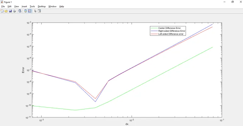
OUTPUT OF THE CODE:
Results:
- Out of three approximation methods, center difference is providing the better results compared to other.
- Center difference approximation uses 5 node-points while Right-sided and left-sided used 6 node-points, so the round off error is less in center difference approximation.
- It is observed the on reducing the dx values the error reduces but after a certain point it starts increasing. This indicated that the value of dx should not be very small and it should be have optimum value.
From the above observations, Central difference gives less error as compared to skewed right and left side difference,but in some cases skewed difference scheme is more useful as compared to central difference. If we want calculate error at boundary,we cannot apply central diiference sheme since it require value from both end so,in this case we can apply skewed diference scheme.