Week 11 - Simulation of Flow through a pipe in OpenFoam
Objective:
The aim of this project is to simulate the flow of water through a pipe and validate the results of the fully developed flow with analytical solutions.
- Validate Hydro-dynamic length with the numerical result
- Validate the fully developed flow velocity profile with its analytical profile
- Validate maximum velocity and pressured drop for fully developed flow
- Post-process Shear stress and validate wall shear stress for fully developed flow.
Problem Definition:
Consider a circular pipe of diameter 100mm and length 12m through which the flowing fluid is water with density of 1000 `(kg)/m^3`. The flow is laminar with a Reynolds number of 2100 & dynamic viscosity of the fluid considered is `10^(-3) "Pa-s"`
Introduction:
The internal flow through the pipe is an axisymmetric problem. Hence the simulation is simplified to a wedge geometry as shown in the figure
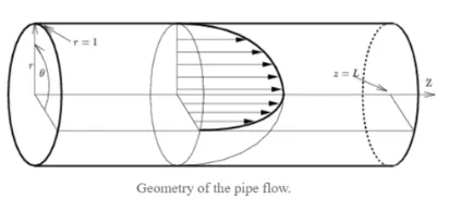
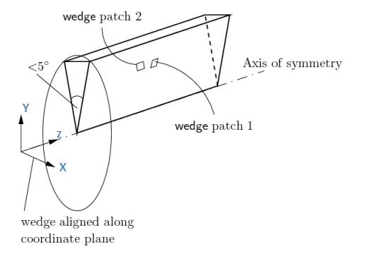
The wedge angle should be limited to a value of 5° to negate the effect of wall curvature. If the angle exceeds the limit of 5°, then the wall curvature should also be taken into account in the simulation. Therefore, here a wedge angle of 5° was used.
Hydrodynamic Entrance Length :-
It is the distance a flow travels in the pipe before it becomes fully developed. Entrance length refers to the length of entry region, the area following the pipe entrance where effects originating from the interior wall of the pipe propagate into the flow as an expanding boundary layer. When the boundary layer expands to fill the entire pipe, the developing flow becomes a fully developed flow, where flow characteristics no longer changes with increased distance along the pipe.
Since the objective of this study is to validate the fully-developed flow simulation, the length of the pipe should be chosen so that it is greater than the hydrodynamic entry length.
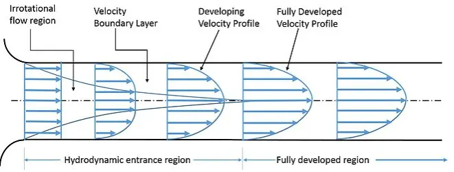
The entrance length depends on the velocity of the fluid, its density and viscosity. For a laminar flow, it can be calculated using the following equation:
`L_(h,Laminar) = 0.05*Re_D*D`
Where `Re_D = (rho*v*D)/(mu) "is the Reynold number of the fluid"`
D - diameter of pipe
`rho - "density of fluid"`
`mu = "dynamic viscosity of fluid"`
`v = "velocity of fluid"`
Preprocessing
The "Block Mesh" utility of OpenFoam was used to generate the Mesh. To generate a wedge geometry. two vertices at the circumference of the wedge should be symmetrical.
A Matlab script was used to generate the blockMeshDict file used in the simulation. It generates the file based on the inputs and it then can be used with OpenFoam.
In order to simulate a 2D case, the number of cells along the z-direction was set to 1. Here the pipe extends in the x-direction.
MATLAB SCRIPT
clc
clear all
close all

%Input Parameters
Re = 2100;
D = 0.1;
r = D/2;
theta = 5;
rho = 1000;
meu = 1e-3;
nu = meu/rho;
v = Re*nu/D; % average velocity
v_max = 2*v; % maximum velocity
A = (pi/4)*D^2; %Area of cross-section
Q = A*v;    %Volumetric flow rate

%Entrance Length
Le = 0.05*Re*D;

%Developed Length
Ld = 1.5;

%Length
L = Le+Ld;

%Analytical Results
%Pressure Drop
deltaP = (8*meu*L*Q)/(pi*r^4)

%Centerline Velocity
v_c = (deltaP*D^2)/(16*meu*L)


%Vertices
xmin = 0;
xmax = L;
ymax = r*cosd(theta/2);
zmin = -r*sind(theta/2);
zmax = r*sind(theta/2);


y = 0:0.001:ymax;

u = @(y) v_c*(1-y.^2/r^2);

plot(y,u(y))


%Nodes
nx=200;
ny=20;
nz=1;

%Grading
gx = 1;
gy = 1;
gz = 1;


line1='/*----------------------------------------*- C++ -*-------------------------------------*\';
line2='|  =========                   |                                                         |';
line3='|  \\      /    F ield         | openFoam: The open source CFD Toolbox                   |';
line4='|   \\    /     O peration     | Website:  https://openfoam.org                          |';
line5='|    \\  /      A nd           | Version:  6                                             |';
line6='|     \\/       M anipulation  |                                                         |';
line7='\\*--------------------------------------------------------------------------------------*/';


f1 = fopen('blockMeshDict.txt','w')
fprintf(f1,'%s\n',line1);
fprintf(f1,'%s\n',line2);
fprintf(f1,'%s\n',line3);
fprintf(f1,'%s\n',line4);
fprintf(f1,'%s\n',line5);
fprintf(f1,'%s\n',line6);
fprintf(f1,'%s\n',line7);

fprintf(f1,'Foamfile\n{\n');
fprintf(f1,'%12s\t 2.0;\n','version');
fprintf(f1,'%11s\t ascii;\n','format');
fprintf(f1,'%10s\t dictionary;\n','class');
fprintf(f1,'%11s\t blockMeshDict;\n','object');
fprintf(f1,'}\n');
line8='//**************************************************************************************//';
fprintf(f1,'%s\n\n',line8);

fprintf(f1,'convertToMeters 1\n\n');
fprintf(f1,'vertices\n(\n');
fprintf(f1,'\t (%f %f %f)\n',xmin,0,0); %point 0
fprintf(f1,'\t (%f %f %f)\n',xmin,ymax,zmax); %point 1
fprintf(f1,'\t (%f %f %f)\n',xmin,ymax,zmin); %point 2
fprintf(f1,'\t (%f %f %f)\n',xmax,0,0); %point 3
fprintf(f1,'\t (%f %f %f)\n',xmax,ymax,zmax); %point 4
fprintf(f1,'\t (%f %f %f)\n',xmax,ymax,zmin); %point 5
fprintf(f1,');\n\n');

fprintf(f1,'blocks\n');
fprintf(f1,'(\n');
fprintf(f1,'\t hex (0 3 5 2 0 3 4 1) (%d %d %d) ',nx,ny,nz);
fprintf(f1,'simpleGrading (%d %d %d)',gx,gy,gz);
fprintf(f1,'\n);\n\n');

fprintf(f1,'edges\n(\n\tarc %d %d (%f %f %f)\n',1,2,0,r,0);
fprintf(f1,'\tarc %d %d (%d %d %d)\n',4,5,L,r,0);
fprintf(f1,');\n\n');


fprintf(f1,'boundary\n(\n');
fprintf(f1,'\t inlet\n');
fprintf(f1,'\t{\n');
fprintf(f1,'\t\t type patch;\n');
fprintf(f1,'\t\t faces\n');
fprintf(f1,'\t\t(\n');
fprintf(f1,'\t\t\t (0 1 2 0)\n');
fprintf(f1,'\t\t );\n');
fprintf(f1,'\t}\n');

fprintf(f1,'\t outlet\n');
fprintf(f1,'\t{\n');
fprintf(f1,'\t\t type patch;\n');
fprintf(f1,'\t\t faces\n');
fprintf(f1,'\t\t (\n');
fprintf(f1,'\t\t\t (3 5 4 3)\n');
fprintf(f1,'\t\t );\n');
fprintf(f1,'\t}\n');

fprintf(f1,'\t top\n');
fprintf(f1,'\t{\n');
fprintf(f1,'\t\t type wall;\n');
fprintf(f1,'\t\t faces\n');
fprintf(f1,'\t\t (\n');
fprintf(f1,'\t\t\t (1 4 5 2)\n');
fprintf(f1,'\t\t );\n');
fprintf(f1,'\t}\n');

fprintf(f1,'\t back\n');
fprintf(f1,'\t{\n');
fprintf(f1,'\t\t type wedge;\n');
fprintf(f1,'\t\t faces\n');
fprintf(f1,'\t\t (\n');
fprintf(f1,'\t\t\t (0 2 5 3)\n');
fprintf(f1,'\t\t );\n');
fprintf(f1,'\t}\n');

fprintf(f1,'\t front\n');
fprintf(f1,'\t{\n');
fprintf(f1,'\t\t type wedge;\n');
fprintf(f1,'\t\t faces\n');
fprintf(f1,'\t\t (\n');
fprintf(f1,'\t\t\t (0 3 4 1)\n');
fprintf(f1,'\t\t );\n');
fprintf(f1,'\t}\n');

fprintf(f1,'\t axis\n');
fprintf(f1,'\t{\n');
fprintf(f1,'\t\t type empty;\n');
fprintf(f1,'\t\t faces\n');
fprintf(f1,'\t\t (\n');
fprintf(f1,'\t\t\t (0 3 3 0)\n');
fprintf(f1,'\t\t );\n');
fprintf(f1,'\t}\n');
fprintf(f1,');\n\n')

fprintf(f1,'mergePatchPairs\n(\n');
fprintf(f1,');\n')


fprintf(f1,'%s\n',line8);

fclose(f1)
blockMeshDict File by File Parsing
/*--------------------------------*- C++ -*----------------------------------*\
  =========                 |
  \\      /  F ield         | OpenFOAM: The Open Source CFD Toolbox
   \\    /   O peration     | Website:  https://openfoam.org
    \\  /    A nd           | Version:  10
     \\/     M anipulation  |
\*---------------------------------------------------------------------------*/
FoamFile
{
    format      ascii;
    class       dictionary;
    object      blockMeshDict;
}
// * * * * * * * * * * * * * * * * * * * * * * * * * * * * * * * * * * * * * //

convertToMeters 1;

vertices
(
	 (0.000000 0.000000 0.000000)
	 (0.000000 0.049952 0.002181)
	 (0.000000 0.049952 -0.002181)
	 (12.000000 0.000000 0.000000)
	 (12.000000 0.049952 0.002181)
	 (12.000000 0.049952 -0.002181)
);

blocks
(
	 hex (0 3 5 2 0 3 4 1) (200 20 1) simpleGrading (1 1 1)
);

edges
(
	arc 1 2 (0.000000 0.050000 0.000000)
	arc 4 5 (12 5.000000e-02 0)
);

boundary
(
	 inlet
	{
		 type patch;
		 faces
		(
			 (0 1 2 0)
		 );
	}
	 outlet
	{
		 type patch;
		 faces
		 (
			 (3 5 4 3)
		 );
	}
	 top
	{
		 type wall;
		 faces
		 (
			 (1 4 5 2)
		 );
	}
	 back
	{
		 type wedge;
		 faces
		 (
			 (0 2 5 3)
		 );
	}
	 front
	{
		 type wedge;
		 faces
		 (
			 (0 3 4 1)
		 );
	}
	 axis
	{
		 type empty;
		 faces
		 (
			 (0 3 3 0)
		 );
	}
);

mergePatchPairs
(
);
//**************************************************************************************//
The solver used is "icoFoam".
Summary of the simulation setup:
|
Parameter |
Value |
|
Number of cells along x |
200">200 |
|
Number of cells along y |
20">200 |
|
Time step size |
0.05s">0.05s |
|
End time |
550s">550s |
controlDict File
/*--------------------------------*- C++ -*----------------------------------*\
  =========                 |
  \\      /  F ield         | OpenFOAM: The Open Source CFD Toolbox
   \\    /   O peration     | Website:  https://openfoam.org
    \\  /    A nd           | Version:  10
     \\/     M anipulation  |
\*---------------------------------------------------------------------------*/
FoamFile
{
    format      ascii;
    class       dictionary;
    location    "system";
    object      controlDict;
}
// * * * * * * * * * * * * * * * * * * * * * * * * * * * * * * * * * * * * * //

application     icoFoam;

startFrom       startTime;

startTime       0;

stopAt          endTime;

endTime         550;

deltaT          0.05;

writeControl    timeStep;

writeInterval   1000;

purgeWrite      0;

writeFormat     ascii;

writePrecision  6;

writeCompression off;

timeFormat      general;

timePrecision   6;

runTimeModifiable true;


// ************************************************************************* //
physicalProperties File
/*--------------------------------*- C++ -*----------------------------------*\
  =========                 |
  \\      /  F ield         | OpenFOAM: The Open Source CFD Toolbox
   \\    /   O peration     | Website:  https://openfoam.org
    \\  /    A nd           | Version:  10
     \\/     M anipulation  |
\*---------------------------------------------------------------------------*/
FoamFile
{
    format      ascii;
    class       dictionary;
    location    "constant";
    object      physicalProperties;
}
// * * * * * * * * * * * * * * * * * * * * * * * * * * * * * * * * * * * * * //

nu              [0 2 -1 0 0 0 0] 1e-6;


// ************************************************************************* //
From the MATLAB Script, the velocity of the fluid is calculated and the same is defined as the boundary condition for inlet velocity.
average velocity at inlet = 0.021 m/s
The boundary condition for outlet is pressure outlet with value 0.
U File
/*--------------------------------*- C++ -*----------------------------------*\
  =========                 |
  \\      /  F ield         | OpenFOAM: The Open Source CFD Toolbox
   \\    /   O peration     | Website:  https://openfoam.org
    \\  /    A nd           | Version:  10
     \\/     M anipulation  |
\*---------------------------------------------------------------------------*/
FoamFile
{
    format      ascii;
    class       volVectorField;
    object      U;
}
// * * * * * * * * * * * * * * * * * * * * * * * * * * * * * * * * * * * * * //

dimensions      [0 1 -1 0 0 0 0];

internalField   uniform (0 0 0);

boundaryField
{
    inlet
    {
        type            fixedValue;
        value		uniform (0.021 0 0);
    }

    outlet
    {
        type            zeroGradient;
    }


    top
    {
        type            noSlip;
    }

    back
    {
    	type		wedge;
    }
    front
    {
    	type		wedge;
    }
    axis
    {
    	type		empty;
    }
}

// ************************************************************************* //
p File
/*--------------------------------*- C++ -*----------------------------------*\
  =========                 |
  \\      /  F ield         | OpenFOAM: The Open Source CFD Toolbox
   \\    /   O peration     | Website:  https://openfoam.org
    \\  /    A nd           | Version:  10
     \\/     M anipulation  |
\*---------------------------------------------------------------------------*/
FoamFile
{
    format      ascii;
    class       volScalarField;
    object      p;
}
// * * * * * * * * * * * * * * * * * * * * * * * * * * * * * * * * * * * * * //

dimensions      [0 2 -2 0 0 0 0];

internalField   uniform 0;

boundaryField
{
    inlet
    {
        type            zeroGradient;
    }

    outlet
    {
        type            fixedValue;
        value 		uniform 0;
    }


    top
    {
        type            zeroGradient;
    }

    back
    {
    	type		wedge;
    }
    front
    {
    	type		wedge;
    }
    axis
    {
    	type		empty;
    }
}

// ************************************************************************* //
POSTPROCESSING
The post processing is done using "paraview".
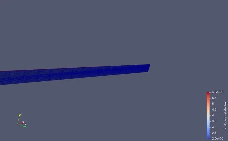
Mesh Output
Mesh near inlet section
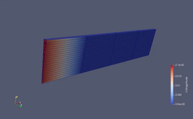
Here inlet and outlet sections are clipped form the pipe.
Mesh near outlet section
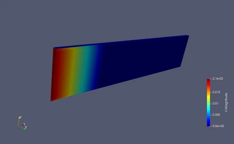
Velocity Output
Near Inlet Section
Near Outlet Section
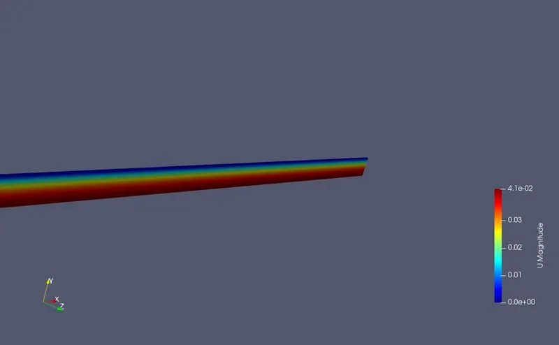
Here inlet and outlet sections are clipped form the pipe.
Results and Discussion:
Since the flow is laminar and incompressible, the icoFOAM solver was chosen in this project. The simulation was carried till an end time of 550 s to allow the flow to become fully developed.
Pressure drop:
From the simulation, the pressure was plotted along the axial direction.
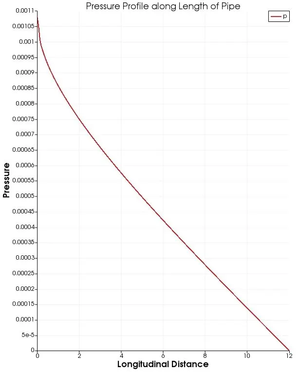
It can be observed that pressure drop decreases along the axial direction. In a horizontal pipe with a constant diameter, the pressure drop is the only force that is driving the flow.
rom the figure, the pressure drop was determined to be 1.1 Pa. Hagen Poiseuille equation can be used to validate the pressure drop obtained from the simulation.
Hagen-Poiseuille equation
According to the Hagen-Poiseuille equation, the pressure drop in a laminar incompressible flow through a cylindrical pipe with constant cross-section is given by
`DeltaP = (8*mu*L*Q)/(pi*R^4)`
where
`Delta P = "pressure drop in the cylindrical pipe in Pa"`
`mu = "dynamic viscosity in P a - s"`
`L = "length of the pipe in m"`
`Q = "volumetric flow rate in " m^3/s`
`R = "adius of the pipe in m"`
Using the above equation in MATALB Script , the prssure drop calculated is 0.806 Pa.
Radial velocity:
In order to quantitatively visualise this development of the flow, the radial velocity profile was plotted in axial or longitudinal direction and at different axial distance (x-distance) in radial direction as shown in the figures below:
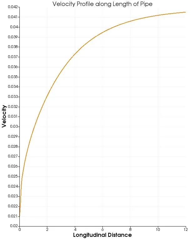
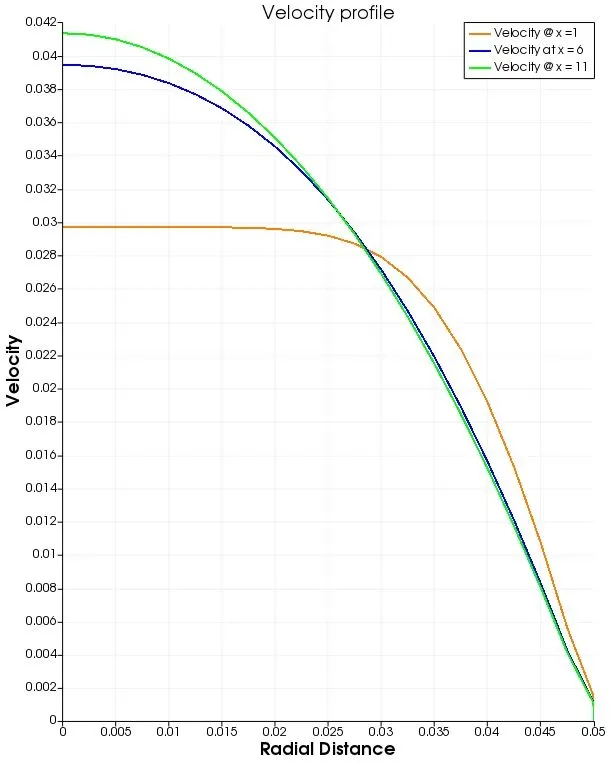
It can be observed that the distance of the velocity profile changes with increasing z-distance and it becomes constant after 10.5 m which is the same as obtained in the previous section. At the exit of the pipe, maximum velocity was found to be 0.04149ms">0.04149m/s at the centre of the pipe.
The analytical velocity profile for a fully developed flow can be obtained from the formula:
`u(r) = V_c*(1-(r^2)/(R^2))`
where
`V_c = (DeltaP*D^2)/(19*mu*L)`
the above forumla is included in MATLAB script.
The simulation result at outlet of pipe are exported as .csv file and imported in MATLAB. The comparison of velocity profile between simulation and analytical results are plotted in MATLAB as showm below:
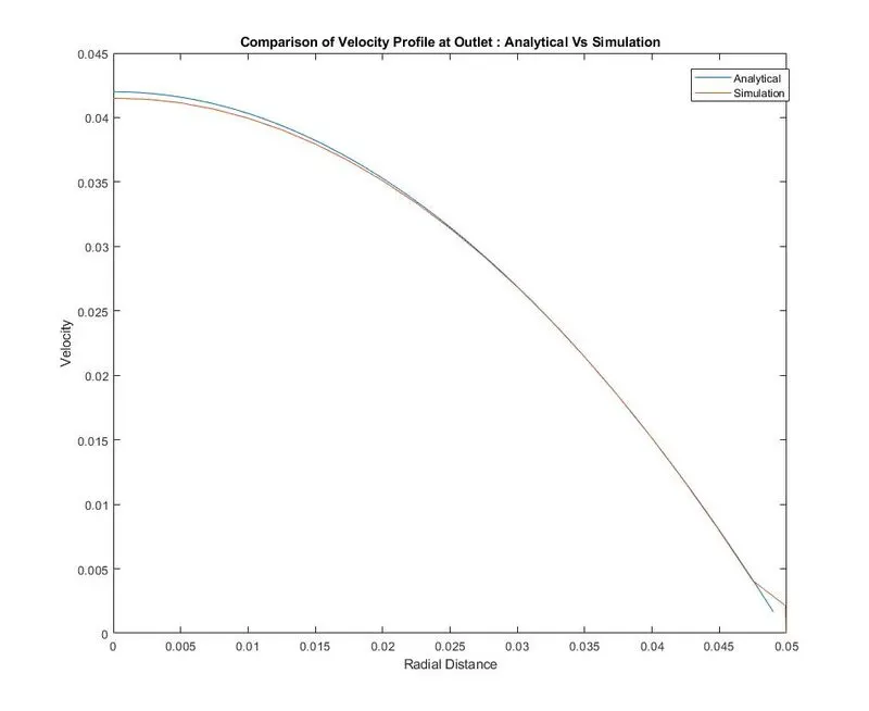
From the above figure, it can be observed that the velocity profile from the simulation is close to the analytical solution.
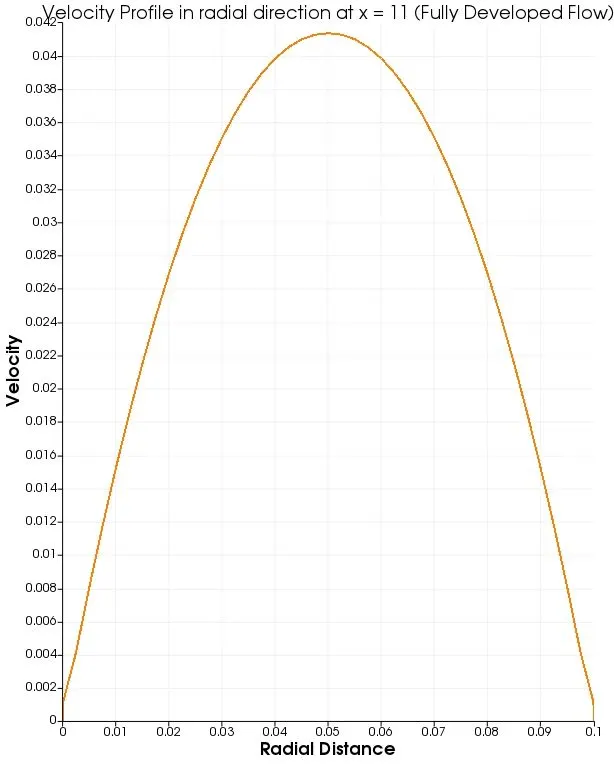
By "refelect" option (Fileters > Alphabetical>Reflect) & choosing the symmetric plane as Y Min in Paraview, the complete 2D solution for fully developed flow (velocity profile along complete diameter) for our probem is visulized by using plot over line tool.
Wall Shear Stress:
In fluids, the wall shear stress is given by
`tau = mu*(du)/(dy)`
From the simulation result,
first, the velocity gradient was determined using the “Gradient of Unstructured Data Set” option in Paraview. Then using "calculator" the dynamic viscosity is multiplied with the gradient to calculate the wall shear stress.
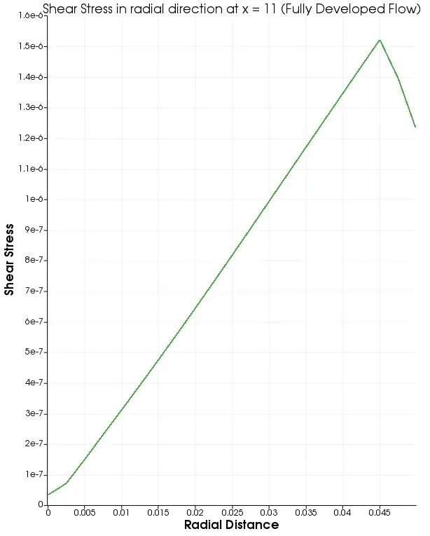
From the above figure, it can be observed that the shear stress increases with the radial distance. So the shear stress is higher near the walls.