Week 9 - FVM Literature Review

In computational fluid dynamics there are 3 numerical method based solvers to solve the governing Navier-strokes equations, Namely,

1. Finite Difference Method

2. Finite Element Method

3. Finite Volume Method

Finite Difference Method:

The grid is linear and aligned so that all grid points lie in a straight line. Mainthing is that the properties are considered to be concentrated at a single point.

Finite Element Method:

The Properties are valid over an elemental area. The properties assumed to be concentrated at area centre.

Finite Volume Method:

• The finite volume method is a method for representing and evaluating partial differential equations in form og algebraic equations.
• In this method, volume itegrates into a partial differential equation that cohtains a divergene term and is converted into surface integrals, using the divergence theorem. These terms are then evaluated as fluxes at surfaces of each finite volume, because the fluxes entering a given finite volume is identical to that leaving the adjacent volume, thus making it conservative.
• 'Finite volume' refers to the small volume surrounding each node point in a mesh.
• The advantage of the finite volume method is that it is easily formulated to allow unstructured meshes and this method is used in many computational fluid dynamic package.

Differences between FDM & FVM:

• A finite difference method (FDM) discretization is based upon the differential form of the PDE to be solved. Each derivative is replaced with an approximate difference formula that can generally be derived from a Taylor series expansion. The computational domain is usually divided into hexagonal cells (grid) and the solution will be obtained at each nodal point.
• A finite volume method (FVM) Discretization is based upon integral form of PDE to be solved (eg. conservation of masses, momentum, or energy). The PDE is written in a form that can be solved for a given finite volume for cells. The computational domain is dicretized into finite volumes and then for every volume , the governing equations are solved. The resulting system of the equations usually involves fluxes of the conserved variables, and thus the calculation of fluxes is very important in FVM.
• The basic advantage of this method over FDM is it does not require the use of structured grids and the effort to convert the given mesh into a structured numerical grid internally is completely avoided.

Lets consider a simple 1-D steady state heat conduction equation with heat generation:

`(del(alpha.(delT)/(delx)))/(delx) + S = 0`

where, S is the source term, `alpha`is the thermal diffusivity term and

`(delT)/(delx)`is temperature gradient along the x-direction.

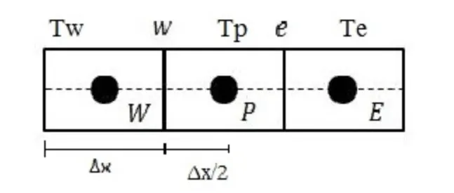
As, the above governing equation is valid at every point in domain, it will also be valid in entire control volume.

If small control volume(dv) is considered and it is multiplied with the governing equation and intergrated it is validated at entire volume and in this entire volume properties are conserved.

Multiplying the equation by 'dv' and integrating it, we finally get:

`alphaA[(T_e-T_p)/(trianglex)]-alpha[(T_e-T_w)/(trianglex)] +S_(avg)dv=0`

where S_avg is the average of the source term and alpha shall not be considered as a function of temperature.

`[Heatflux]_(OUT)-[Heatflux]_(IN)+Source term=0`

The amount of heat that is removed fro a particular box is conserved.

Different schemes used to solve the equation:

1.Gradient scheme

2.Interpolation Scheme

1. Gradient Scheme

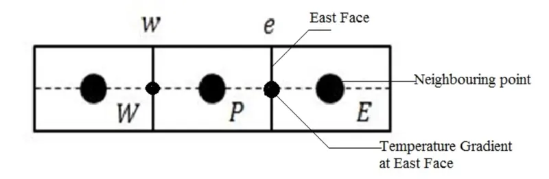
From the above figure, to calculate temperature gradient in the east face, we basically use temperature from neighbouring point trying to evaluate or numerically represent gradient of temperature

Interpolation Schemes:

In FVM formulation, evaluation of surface and volume integrals may require values of the variabe at locations other than the computational nodes of the CV. values at these locations are obtained using interpolation fomrulae. In the same example as above, to integrate the governing equation over the CV around grid point P, needs values of east and west faces, evaluate. Thus, using certian interpolation schemes, we shall evaluate them effectively.

Upwind Interpolation:

The upwind interpolation (UDS) for approximating the value of a variable at the east face of a control volume is given by:

`f_e = f_p, if (v.n)_e >0; f_e if (v.n)_e <0`

This interpolation scheme is equivalent to using a backward or forward finite difference approximation (deoending on the flow direction).

Linear Interpolation (CDS):

We can approximate the value of the variable at the CV face center by linear interpolation of the values at the two nearest computational nodes. Thus, at location 'e' on a cartesian grid, the variable value is approximated by;

`f_e =f_Elambda_e + f_p(1-lambda_e),`

`Lambda_e =(x_e -x_p)/(x_E-x_p)`

The linear interpolational is equivalent of the use of the central difference formula of the use of the central differenc formula of the first-order derivative, and hence, this scheme is also termed as central difference scheme (CDS). This scheme is second-order accurate and may produce oscillatory solution.

Quadratic upwind interpolation (quick):

Quadratic upwind interpolation scheme can be derived using polynomial fitting. The QUICK interpolation on a uniform cartesian grid is given by ;

`phi_e =6/8phi_U+3/8phi_D-1/8phi_(UU)`

where D,U and UU denote the downstream, the first upstream, and the second upstram node respectively (E,P and W or P,R and EE depending o the flow direction). The QUICK scheme is third-order accurate, but prone to oscillations.

Also, there are two more interpolation schemes namely, Hybrid scheme and Total variation Diminishing (TVD) scheme. In addition to these Gradient scheme and Interpolation schemes there are Flux Limiters.

Fux limiters:

Flus limiters are used in the high-resolution scheme used to solve the problem in science and engineering, particularly fluid dynamics described by PDE's. They are used in a high-resolution scheme such as the MUSCL scheme to avoid the spurious oscillation that would otherwise occur with high order spatial discretization scheme due to shocks, discontinuities, or sharp changes in the solution domain. The use of flux limiters together with an appropriate high resolution scheme makes the solution's total variation diminishing (TVD).

The main idea behind the construction of flux limiters scheme is to limiit the spatial derivatives to realistic values for scientific and engineering problems this usually means physically realizable and meaningful value. they are used in high resolution scheme for solving problems described by PDEs and only come into operation when sharp wavefronts are present. For smootl chnaging waves, the flux limiters do not operate, and the spatial derivatives can be represented by high-order approximation without introducing spurious oscillations.

Consider the 1D semi-discrete scheme below:

`(du_i)/(dt) + 1/(trianglex_i)[F(u_(i+1/2))-F(u_(i-1/2))] =0,`

where,

`F(u_(i+1/2)) and F(u_(i-1/2))` represents low and high resolution schemes, then the flux limiters can be switch between these schemes depending upon the gradient close to a particular cell as follows;

`F(u_(i+1/2)) =f_(i+1/2)^(low) - phi(r_i)(f_(i+1/2)^(low)-f_(i+1/2)^(high))`

`F(u_(i-1/2)) =f_(i+1/2)^(low) - phi(r_(i-1))(f_(i-1/2)^(low)-f_(i-1/2)^(high))`

where.\,`f^(low)` is low resolution flux and `f^(high)` is high resolution flux

`phi(r)`is the flux limiter function and r represent the ratio of successive gradients on solution mesh.

`r_i =(u_i-u_(i-1))/(u_(i+1)-u_i)`

The limiter function is contrained to be greater or equal to zero the flux is represented by a low resolution scheme. Similarly, when the limiter is equal to 1 it is represented by a high resolution scheme. The various limiters have differing switching characteristics and selected acording to the particular problem and solution scheme.