Week 3.5 - Deriving 4th order approximation of a 2nd order derivative using Taylor Table method

Objective:

To compute and compare the truncation error in the numerically derived solutions of a second order derivative using the fourth order approximation of central, right sided skewed and left sided skewed differences methods with that of the solution derived analytically, using MATLAB

Theory:

Talyor series is often useful in physical situations and are known for it's ease to numerical operate any nasty function to any degree of accuracy. There several methods to utilise the theory of Taylor series and here we are going look into three important schemes in the Taylor series approximation method, that are basically classified based on the position of the grid points with respect to initial point used for inputs -

(i) central differences scheme- uses the equal number of grid points that ahead and behind of the initial point 'i' and the expression for fourth order approcimation of second order derivative utilising the central differences scheme is as follows:

`del^2x`/`delt^2``approx` `(a_1*f_(i-2) + b_1*f_(i-1) + c_1*f_(i) + d_1*f_(i+1) + e_1*f_(i+2)) / (trianglex)^2`

The number of grid points can be determinder for a central differences scheme with a simple formula = p+q-1, where p is the order of the derivative & q is the order of approximation, thus for our case, we need (2+4-1)=5 grid points, hence, 5 grid points - 'i-2','i-1','i','i+1','i+2'.

(ii) Right sided skewed scheme - uses the grid points that are on the right side/ ahead of the initial point 'i' and the fourth order approximation of a second order derivative in this scheme can be expressed as follows

`del^2x`/`delt^2``approx` `(a_2*f_(i) + b_2*f_(i+1) + c_2*f_(i+2) + d_2*f_(i+3) + e_2*f_(i+4)+g_2*f_(i+5)) / (trianglex)^2`

For this scheme,the number of grid points required is calculated using a simple formula = p+q, where p is the order of the derivative & q is the order of approximation, thus for our case, we need (2+4)=6 grid points, hence, 6 grid points -'i','i+1','i+2','i+3','i+4','i+5' .

(iii) Left sided skewed scheme - uses the grid points that are on the left side/ behind of the initial point 'i' and the fourth order approximation of a second order derivative in this scheme can be expressed as follows

`del^2x`/`delt^2``approx` `(a_3*f_(i) + b_3*f_(i-1) + c_3*f_(i-2) + d_3*f_(i-3) + e_3*f_(i-4)+g_3*f_(i-5)) / (trianglex)^2`

For this scheme,the number of grid points required is calculated using a simple formula = p+q, where p is the order of the derivative & q is the order of approximation, thus for our case, we need (2+4)=6 grid points, hence, 6 grid points -'i','i-1','i-2','i-3','i-4','i-5' .

The constants in the above equations are derived using the Taylors table and are computed in the program below.

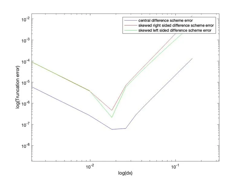
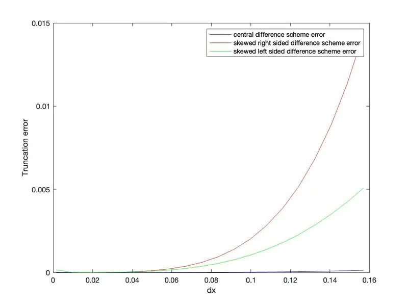
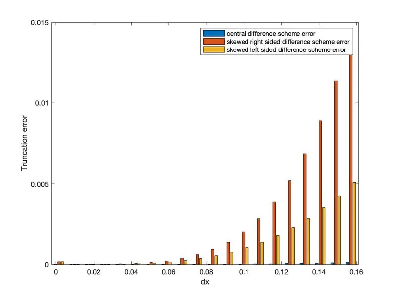
The following code computes the constants in the above equation that is derived from the Taylors table, then uses them to compute and compare the truncation error in the numerically derived solutions of a second order derivative using the fourth order approximation of central, right sided skewed and left sided skewed differences methods with that of the solution derived analytically and also shows how the errors decay w.r.t the size of the dx.

Main script:

clear all
close all
clc

%given function: f(x)=(e^x)*cos(x)
%analytical second order derivative of f(x): f"(x)=-2*sin(x)*(e^x)
%analytical_derivative=-2*sin(x)*(e^x);

%central differencing scheme
%f"(x)=[af(x-2dx)+bf(x-dx)+cf(x)+df(x+dx)+ef(x+2dx)]/((dx)^2)
%using Taylor Table we get the constants
AC=[1,1,1,1,1;
   -2,-1,0,1,2;
   2,1/2,0,1/2,2;
   -4/3,-1/6,0,1/6,4/3;
   2/3,1/24,0,1/24,2/3;
   -4/15,-1/120,0,1/120,4/15];
K = [0;0;1;0;0;0];
%X_center=[a;b;c;d;e;g];
XC=vpa(linsolve(AC,K),3);
C=vpa(ACK,3);
t1=num2cell(C);
[a1,b1,c1,d1,e1]=deal(t1{:})
AF=[1,1,1,1,1,1;
    0,1,2,3,4,5;
    0,1/2,2,9/2,8,25/2;
    0,1/6,4/3,9/2,32/3,125/6;
    0,1/24,2/3,27/8,32/3,625/24;
    0,1/120,4/15,243/120,128/15,625/24];
XF= vpa(linsolve(AF,K),3);
F=vpa(AFK,3);
t2=num2cell(F);
[a2,b2,c2,d2,e2,g2]=deal(t2{:})
AB=[1,1,1,1,1,1;
    0,-1,-2,-3,-4,-5;
    0,1/2,2,9/2,16/2,25/2;
    0,-1/6,-8/6,-27/6,-64/6,-125/6;        
    0,1/24,16/24,27/8,32/3,625/24;
    0,-1/120,-32/120,-243/120,-1024/120,-3125/120];
XB= vpa(linsolve(AB,K),3);
B=vpa(ABK,3);
t3=num2cell(B);
[a3,b3,c3,d3,e3,g3]=deal(t3{:})

%inputs(assumed)
x=pi/3;
dx=linspace(pi/20,pi/2000,20);

for i=1:length(dx)
    [central_diff_error(i),skewed_right_error(i),skewed_left_error(i)]=fourth_order_approx_err(x,dx(i),a1,b1,c1,d1,e1,a2,b2,c2,d2,e2,g2,a3,b3,c3,d3,e3,g3);
end

figure(1)
title('decay of truncation error wrt size of dx');
loglog(dx,central_diff_error,'blue')
hold on
loglog(dx,skewed_right_error,'red')
hold on
loglog(dx,skewed_left_error,'green')
legend('central difference scheme error','skewed right sided difference scheme error','skewed left sided difference scheme error');
xlabel('log(dx)'); ylabel('log(Truncation error)');
axis auto;

figure(2)
title('decay of truncation error wrt size of dx');
plot(dx,central_diff_error,'blue')
hold on
plot(dx,skewed_right_error,'red')
hold on
plot(dx,skewed_left_error,'green')
legend('central difference scheme error','skewed right sided difference scheme error','skewed left sided difference scheme error');
xlabel('dx'); ylabel('Truncation error');
axis auto;

figure(3)
bar(dx,[central_diff_error;skewed_right_error;skewed_left_error])
xlabel('dx'); ylabel('Truncation error')
legend('central difference scheme error','skewed right sided difference scheme error','skewed left sided difference scheme error');
axis auto

Function code:

function [central_diff_error,skewed_right_error,skewed_left_error] = fourth_order_approx_err(x,dx,a1,b1,c1,d1,e1,a2,b2,c2,d2,e2,g2,a3,b3,c3,d3,e3,g3)

%analytical function: f(x)= exp(x)*cos(x)
analytical_derivative =-2*sin(x)*exp(x);

%Central diff approximation
central_diff= (a1*exp(x-2*dx)*cos(x-2*dx)+b1*exp(x-dx)*cos(x-dx)+c1*exp(x)*cos(x)+d1*exp(x+dx)*cos(x+dx)+e1*exp(x+2*dx)*cos(x+2*dx))/(dx)^2;
%second order difference approximation
skewed_right_diff= (a2*exp(x)*cos(x) + b2*exp(x+dx)*cos(x+dx) + c2*exp(x+2*dx)*cos(x+2*dx) + d2*exp(x+3*dx)*cos(x+3*dx) + e2*exp(x+4*dx)*cos(x+4*dx) + g2*exp(x+5*dx)*cos(x+5*dx))/(dx)^2;
%fourth order difference approximation
skewed_left_diff=(a3*exp(x)*cos(x) + b3*exp(x-dx)*cos(x-dx) + c3*exp(x-2*dx)*cos(x-2*dx) + d3*exp(x-3*dx)*cos(x-3*dx) + e3*exp(x-4*dx)*cos(x-4*dx) + g3*exp(x-5*dx)*cos(x-5*dx))/(dx)^2;
%error in first order diff approx
central_diff_error=abs(central_diff-analytical_derivative);
%error in second order diff approx
skewed_right_error=abs(skewed_right_diff-analytical_derivative);
%error in fourth order diff approx
skewed_left_error=abs(skewed_left_diff-analytical_derivative);

end

Results:

Conclusion:

From the graph it is evident that the central differencing scheme is better than the other two in terms of accuracy. The inflation in the error after an optimal step size'dx' shows that higher order terms are reproducing infinitesmal truncation erros which aren't stable and may be a factor few other parameters, which are usually eliminated by chosing appropriate range of step size. Despite the fact that the order of accuracy isnt better for the skewed schemes, the biggest advantage of the Skewed schemes over the central diff scheme is that central differences scheme wont be useful at the boundary, as we will be able to use grids of only one side and thus, skewed schemes are particularly useful when at boundary. Though there are forward or backward approximations, they dont favour the order of approximations comparitively, causing more errors.