Week 7 - Simulation of a 1D Super-sonic nozzle flow simulation using Macormack Method

Objectives:

• Compute, simulate and compare the flow through a supersonic nozzle using both conservative and non conservative governing equations to solve.
• perform the computation using Macormack explicit difference method to solve both the conservative and non conservative forms of the governing equation for a flow through a supersonic nozzle and also to perform grid dependence test.
• To show the Steady-state distribution of primitive variables ,Time-wise variation of the primitive variables inside nozzle, Variation of Mass flow rate distribution inside the nozzle at different time steps during the time-marching process and comparre the Normalized mass flow rate distributions of both forms and make suitable conclusions based on these.

Theory:

1D Supersonic nozzle flow:

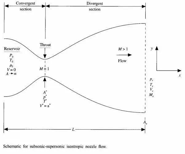
The nozzle has a convergent, throat and a divergent section In convergent section when mach no. is less than 1(M<1), this condition is called subsonic flow through nozzle and here the flow starts to converge and at the throat the flow reaches mach 1 and after with the expansion in the divergent section, the flow expands and will become supersonic,i.e.,M>1. Mach number is a dimensionless quantity representing the ratio of flow velocity past a boundary to the local speed of sound.

`M=v/c`, where v is the velocity of the particle or any object and c is the speed of the sound at a given altitude.

Assuming air to be an ideal gas, the formula to compute Mach number in a subsonic compressible flow is as follows:

`M=sqrt((2/(gamma-1)((q_c/p+1)^((gamma-1)/gamma)-1)`

and the speed of the sound is given by: `c=sqrt(gammaRT)`

where , `q_c`- dynamic pressure, p-static pressure, `gamma`-ratio of specific heat, R- specific gas constant of air

Quasi 1D flow:

A quasi one-dimensional flow is one in which all variales vary primarily along one direction, say x. A flow in a duct with slowly varying area A(x) is our case here, which has the physical meaning that the slope of the duct walls is small and also that the velocity component in x direction will be dominant than that in the y and z direction.

Mac-Cormak method:

To discretize the numerical solution we use the technique called Maccormack method. The MacCormack method is a variation of the two-step Lax-Wendroff scheme but is much simpler in application. The application of MacCormack method proceeds in two steps; a predictor step which is followed by a corrector step.In the predictor step, we use the forward differencing scheme and update the solution to use it in the corrector step. Corrector step uses a backward diffencing scheme and update the solution with the average of the solutions from both the steps.

Governing equations of 1D quasi suoersonic nozzle flow:

Governing equations are of two types:

1. Conservative form

2. Non conservative form

Non conservative form:

1. Continuity:

`(del(rho))/(del(t)) = -rho*(del(V))/(del(x))-rho*V*(del(lnA))/(del(x))-V*(del(rho))/(del(x))`

2. Momentum:

`(delV)/(delt)=-V*(delV)/(delx)-(1/gamma)*(((delT)/(delx) +(T/rho)*(delrho)/(delx))`

3. Energy:

`(delT)/(delt)=-V*(delT)/(delx)-(gamma-1)*T*((delV)/(delx)+(V)*(del(lanA))/(delx))`

Calculation of time step:

In this solution, the time step is calculated based Courant number, with the following relation:

`dt=C*(dx/(a+V))`

With this relation we calculate dt at each node and then the minimum value of all dt will be considered.

Boundary conditions:

At the inlet, the flow variables such as temperature and density remain constant and the value of veloity change.

`v_1=2*v_2-v_3`

At outlet conditions, all the flow variables keep on changing

`v_n=2*v_(n-1)-v_(n-2)`

`rho_n=2*rho_(n-1)-rho_(n-2)`

`T_n=2*T_(n-1)-T_(n-2)`

Initial conditions:

Area, A=1+2.2*(x-1.5)^2

Density, `rho`=1-(0.3146*x)

Temperature, T =1-(0.2314*x)

Velocity, V=(0.1+(1.09*x))*(T^0.5)

Conservative form:

The equations for Quasi 1D flow are expressed in the generic form. the equations consists of solution vector U and the flux vector F and the Source term j as follows.

`U_1=rho'A'`

`U_2=rho'A'V'`

`U_3=rho'((e')/(gamma-1)+gamma/2V'^2)A'`

`F_1=rho'A'V'`

`F_2=rho'A'V'^2+1/gammarho'A'`

`F_3=rho'((e')/(gamma-1)+gamma/2V'^2)V'A'+rho'A'V'`

`J_2=1/gammarho'(delA')/(delx')`

With the help of the above elements, solution vector equations can be written as

`(delU_1)/(delt')=-(delF_1)/(delx')`

`(delU_2)/(delt')=-(delF_2)/(delx')+J_2`

`(delU_3)/(delt')=-(delF_3)/(delx')`

Once the above quations are solved numerically, we get the results for solution vector U(`U_1,U_2,U_3`) in steps of time and in order to obatain the primitive variables density, velocity,Temperature and pressure solutions vector must be decoded.

`rho'=U_1/(A')`

`V'=U_2/U_1`

`T'=e'=(gamma-1)(U_3/U_1-gamma/2V'^2)`

`rhoi'=rho'T'`

Boundary conditions:

At Inlet boundary, U1 stays fixed and other two solution vector U2 and U3 will float with respect to time, thus,

U1=`rho(1)A(1)`

U2=2*U2-U3

`U3=U1*((T/(gamma-1))+((gamma/2)*(sqrt(v))))`

At outlet bounary, U1, U2 & U3 will be changing with time

U1(n)=2*U1(n-1)-U1(n-2)

U2(n)=2*U2(n-1)-U2(n-2)

U3(n)=2*U3(n-1)-U3(n-2)

Initial Conditions:

Area, A=1+2.2*(x-1.5)^2, it remains constant through out the nozzle

Velocity, `v=-0.59/(rho*A)`

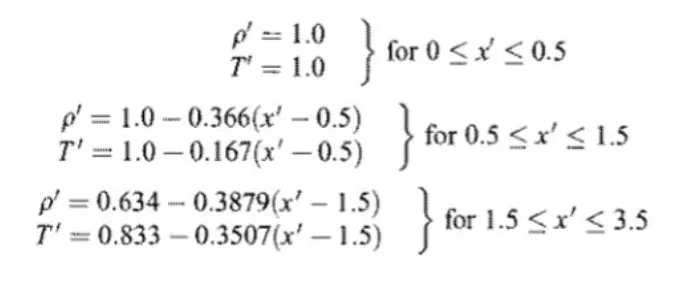
At t=0, values of density and temperature throughout the nozzle are given as follows:

MATLAB code:

Main script:

clear all
close all
clc

%Inputs
L=3; %Domain length
n=31;%no. grid points
%th=(n+1)/2;% grid position of throat
x=linspace(0,L,n);
dx=x(2)-x(1);%mesh
%rho_stag=1; temp_stag=1;
g =1.4;%gamma
%M=0;
A=1+(2.2*(x-1.5).^2);%Area
%b=a*-1;
C=0.5;%CFL number
nt=1400;%no. of time steps
t_array=1:nt;

%solution for non conservative form:
tic;
[m,M,v,T,P,rho,T_th,rho_th,P_th,M_th]=NC_solver(x,dx,n,C,g,nt);
sim_time_NC=toc;
fprintf('The computation time for non conservative form =%f',sim_time_NC);

%Time wise variation of mach number density, pressure and temparature for Non-consrvative form
Time_variation=figure(2)
subplot(4,1,1)
plot(t_array,rho_th);
xlabel('Time')
ylabel('Density');

subplot(4,1,2)
plot(t_array,T_th);
xlabel('Time')
ylabel('Temperature');

subplot(4,1,3)
plot(t_array,P_th);
xlabel('Time')
ylabel('pressure');

subplot(4,1,4)
plot(t_array,M_th);
xlabel('Time')
ylabel('Mach number');

%legend('density','temperature','pressure','Mach number');

%Qualitative aspect of 1D supersonic nozzle flow: Non conservative from:
Qualitative_C=figure(3)
subplot(4,1,1)
plot(x,rho);
xlabel('x')
ylabel('Density');

subplot(4,1,2)
plot(x,T);
xlabel('x')
ylabel('Temperature');

subplot(4,1,3)
plot(x,P);
xlabel('x')
ylabel('pressure');

subplot(4,1,4)
plot(x,M);
xlabel('x')
ylabel('Mach number');

%solution for conservative form:
tic;
[m_c,M_c,v_c,T_c,P_c,rho_c,T_th_c,rho_th_c,P_th_c,M_th_c]=cons_solver(x,dx,n,C,g,nt);
sim_time_C=toc;
fprintf('The computation time for non conservative form =%f',sim_time_C);

%Time wise variation of mach number density, pressure and temparature for consrvative form
Time_variation=figure(4)
subplot(4,1,1)
plot(t_array,rho_th_c);
xlabel('Time')
ylabel('Density');

subplot(4,1,2)
plot(t_array,T_th_c);
xlabel('Time')
ylabel('Temperature');
subplot(4,1,3)
plot(t_array,P_th_c);
xlabel('Time')
ylabel('pressure');

subplot(4,1,4)
plot(t_array,M_th_c);
xlabel('Time')
ylabel('Mach number');

%Qualitative aspect of 1D supersonic nozzle flow: conservative from:
Qualitative_C=figure(5)
subplot(4,1,1)
plot(x,rho_c);
xlabel('x')
ylabel('Density');

subplot(4,1,2)
plot(x,T_c);
xlabel('x')
ylabel('Temperature');

subplot(4,1,3)
plot(x,P_c);
xlabel('x')
ylabel('pressure');

subplot(4,1,4)
plot(x,M_c);
xlabel('x')
ylabel('Mach number');

figure(7)
plot(x,m)
hold on
plot(x,m_c)
hold on
xlabel('x')
ylabel('Mass flow rate')
legend('Non conservative form','Conservative form')

function code for non conservative form:

function [m,M,v,T,P,rho,T_th,rho_th,P_th,M_th]=NC_solver(x,dx,n,C,g,nt)

%Initial conditions(at t=0)

rho_i=1-0.3146*x;%Density
T_i=1-0.2314*x;%Temperature
v_i=(0.1+1.09*x).*(T_i.^0.5);%velocity
A=1+(2.2*(x-1.5).^2);%Area
%nd_x=x/L
%Fielf variables
rho=rho_i;T=T_i;v=v_i;

a=sqrt(T);%sonic velocity
P=rho.*T;%pressure ratio
M=v./(T.^0.5);%Mach number
m=rho.*v.*A;%Mass flow rate
%stencil metrics for throat section
th=find(A==1);

%calculating time step

 for i=1:n
     dt_calc(i)=(C*dx)/(a(i)+v(i));
 end
dt=min(dt_calc);

%outer time loop
for k=1:nt

%     dt=min(C.*dx./(a+v));
    %initial conditions as old conditions
    rho_old=rho; T_old=T;v_old=v;

    %predictor step
    for i=2:n-1
        drho_dx=(rho(i+1)-rho(i))/dx;
        dv_dx=(v(i+1)-v(i))/dx;
        dT_dx=(T(i+1)-T(i))/dx;
        dlogA_dx= (log(A(i+1))-log(A(i)))/dx;             

        %continuity equation
        drho_dt_p(i)=-(rho(i)*dv_dx) - (rho(i)*v(i)*dlogA_dx) - (v(i)*drho_dx);

        %Momentum equation
        dv_dt_p(i)=-(v(i)*dv_dx) - ((1/g)*(dT_dx + (T(i)*drho_dx/rho(i))));        

        %Energy equation
        dT_dt_p(i)= -(v(i)*dT_dx) - ((g-1)*T(i)*(dv_dx + (v(i)*dlogA_dx)));

        %solution update
        rho(i)=rho(i)+drho_dt_p(i)*dt;
        v(i)=v(i)+dv_dt_p(i)*dt;
        T(i)=T(i)+dT_dt_p(i)*dt;
    end

    %corrector step
    for i=2:n-1
        drho_dx=(rho(i)-rho(i-1))/dx;
        dv_dx=(v(i)-v(i-1))/dx;
        dT_dx=(T(i)-T(i-1))/dx;
        dlogA_dx= (log(A(i))-log(A(i-1)))/dx;           

        %continuity equation
        drho_dt_c(i)=-(rho(i)*dv_dx) - (rho(i)*v(i)*dlogA_dx) - (v(i)*drho_dx);

        %Momentum equation
        dv_dt_c(i)=-(v(i)*dv_dx) - ((1/g)*(dT_dx + (T(i)*drho_dx/rho(i))));         

        %Energy equation
        dT_dt_c(i)= -(v(i)*dT_dx) - ((g-1)*T(i)*(dv_dx + (v(i)*dlogA_dx)));

    end
    %Averaging the time derivatives
    drho_dt_avg=0.5*(drho_dt_p+drho_dt_c);
    dv_dt_avg=0.5*(dv_dt_p+dv_dt_c);
    dT_dt_avg=0.5*(dT_dt_p+dT_dt_c);

    % final solution update
    for i=2:n-1
        rho(i)=rho_old(i)+drho_dt_avg(i)*dt;
        v(i)=v_old(i)+dv_dt_avg(i)*dt;
        T(i)=T_old(i)+dT_dt_avg(i)*dt;
    end

    %Applying BC
    %Inlet
    v(1)=2*v(2)-v(3);
    %outlet
    v(n)=2*v(n-1)-v(n-2);
    rho(n)=2*rho(n-1)-rho(n-2);
    T(n)=2*T(n-1)-T(n-2);

    P=rho.*T;%pressure ratio
    a=sqrt(T);
    M=v./a;%Mach number
    m=rho.*v.*A;%Mass flow rate

    %initializing index for updation of primitive variable at throat wrt to
    %increment in time step
    rho_th(k)=rho(th);
    T_th(k)=T(th);
    P_th(k)=P(th);
    M_th(k)=M(th);
    v_th(k)=v(th);
    m_th(k)=m(th);


    %Comparision of non dimensional mass flow rates at different time:
    mass=figure(1);
    if k==50
        plot(x,m,'linewidth',1.75);
        hold on
    elseif k==100
        plot(x,m);
        hold on
    elseif k==200
        plot(x,m);
        hold on
    elseif k==400
        plot(x,m);
        hold on
    elseif k==700
        plot(x,m);
        hold on
    elseif k==900
        plot(x,m);
        hold on
    elseif k==1200
        plot(x,m);
        plot(x(end),m(end));
        hold on
    end
end

title('Comparision of Non-Dimensional mass flow rates at different time instances');
xlabel('x/L (Non-Dimensional distance through the nozzle');
ylabel('ND mass flow rate');
legend('50deltat','100deltat','200deltat','400deltat','700deltat','900deltat','1200deltat');
axis([0 3 0 2.5]);
grid on;
grid minor;

function code for Conservative form:

function [m_c,M_c,v_c,T_c,P_c,rho_c,T_th_c,rho_th_c,P_th_c,M_th_c]=cons_solver(x,dx,n,C,g,nt)

A=1+(2.2*(x-1.5).^2);
th=find(A==1);%throat profile
for i=1:n
    if x(i)<=0.5
        rho_c(i) = 1;
        T_c(i) =1;
        v_c(i) = 0.59/(rho_c(i)*A(i));

    end
    if  x(i)>0.5 && x(i)<1.5
        rho_c(i) = 1-(0.366*(x(i)-0.5));
        T_c(i) = 1-(0.167*(x(i)-0.5));
        v_c(i) = 0.59/(rho_c(i)*A(i));
    end
    if x(i)>=1.5
        rho_c(i) = 0.634-(0.3879*(x(i)-1.5));
        T_c(i) = 0.833-(0.3507*(x(i)-1.5));
        v_c(i) = 0.59/(rho_c(i)*A(i));
    end
end
a=sqrt(T_c);
U1 = rho_c.*A;
U2 = U1.*v_c;
U3 = U1.*((T_c./(g-1)) +((g/2)*v_c.^2));

v_c = v_c;
%outer time loop
for k=1:nt

    dt=min(C.*dx./(a+v_c));%time step
    U1_old=U1;
    U2_old=U2;
    U3_old=U3;

    %Calculatingthe Flux vector(F)
    F1=U2;
    F2=((U2.^2)./U1)+((g-1)/g)*(U3-(g/2)*((U2.^2)./U1));
    F3=((g*U2.*U3)./U1)-(g*(g-1)*(U2.^3)./(2*U1.^2));

    %predictor step
    for i=2:n-1

        %Calculating the source terms:
        J2=(1/g)*rho_c(i)*T_c(i)*(A(i+1)-A(i))/dx;

        %continuity equation
        dU1_dt_p(i)=-(F1(i+1)-F1(i))/dx;
        %Momentum equation
        dU2_dt_p(i)=(-(F2(i+1)-F2(i))/dx)+J2;
        %Energy equation
        dU3_dt_p(i)= -(F3(i+1)-F3(i))/dx;
        %solution update
        U1(i)=U1(i)+dU1_dt_p(i)*dt;
        U2(i)=U2(i)+dU2_dt_p(i)*dt;
        U3(i)=U3(i)+dU3_dt_p(i)*dt;
    end

    %Updating flux vectors
    F1=U2;
    F2=((U2.^2)./U1)+((g-1)/g)*(U3-(g/2)*((U2.^2)./U1));
    F3=((g*U2.*U3)./U1)-(g*(g-1)*(U2.^3)./(2*U1.^2));
    rho_c=U1./A;
    v_c=U2./U1;
    T_c=(g-1)*((U3./U1-(g/2)*(v_c).^2));


    %corrector step
    for i=2:n-1

        %Updating the source terms:
        J2=(1/g)*rho_c(i)*T_c(i)*(A(i)-A(i-1))/dx;

        %continuity equation
        dU1_dt_c(i)=-(F1(i)-F1(i-1))/dx;
        %Momentum equation
        dU2_dt_c(i)=-((F2(i)-F2(i-1))/dx)+J2;
        %Energy equation
        dU3_dt_c(i)= -(F3(i)-F3(i-1))/dx;
    end
    %Averaging the time derivatives
    dU1_dt_avg=0.5*(dU1_dt_p+dU1_dt_c);
    dU2_dt_avg=0.5*(dU2_dt_p+dU2_dt_c);
    dU3_dt_avg=0.5*(dU3_dt_p+dU3_dt_c);

    % final solution update
    for i=2:n-1
        U1(i)=U1_old(i)+dU1_dt_avg(i)*dt;
        U2(i)=U2_old(i)+dU2_dt_avg(i)*dt;
        U3(i)=U3_old(i)+dU3_dt_avg(i)*dt;
    end
% 
%     %Final Primitive value update
%     rho_c=U1./A;
%     v_c=U2./U1;
%     T_c=(g-1)*((U3./U1-(g/2)*(v_c).^2));

    P_c=rho_c.*T_c;%pressure ratio
    M_c=v_c./(sqrt(T_c));%Mach number
    m_c=rho_c.*A.*v_c;%Mass flow rate

    %Applying BC
    %Inlet
    U1(1)=rho_c(1)*A(1);
    U2(1)=2*U2(2)-U2(3);
    v_c(1)=U2(1)./U1(1);
    U3(1)=U1(1)*((T_c(1)/(g-1))+((g/2)*(v_c(1)).^2));
    %outlet
    U2(n)=2*U2(n-1)-U2(n-2);
    U1(n)=2*U1(n-1)-U1(n-2);
    U3(n)=2*U3(n-1)-U3(n-2);
    rho_c=U1./A;
    v_c=U2./U1;
    T_c=(g-1)*((U3./U1-(g/2)*(v_c).^2));


    %initializing index for updation of primitive variable at throat wrt to
    %increment in time step
    rho_th_c(k)=rho_c(th);
    T_th_c(k)=T_c(th);
    P_th_c(k)=P_c(th);
    M_th_c(k)=M_c(th);
    v_th(k)=v_c(th);
    m_th(k)=m_c(th);


    %Comparision of non dimensional mass flow rates at different time:
    mass=figure(6);
    if k==50
        plot(x,m_c,'linewidth',1.75);
        hold on
    elseif k==100
        plot(x,m_c);
        hold on
    elseif k==200
        plot(x,m_c);
        hold on
    elseif k==400
        plot(x,m_c);
        hold on
    elseif k==700
        plot(x,m_c);
        hold on
    elseif k==900
        plot(x,m_c);
        hold on
    elseif k==1200
        plot(x,m_c);
        plot(x(end),m_c(end));
        hold on
    end
end

title('Comparision of Non-Dimensional mass flow rates at different time instances');
xlabel('x/L (Non-Dimensional distance through the nozzle');
ylabel('ND mass flow rate');
legend('50deltat','100deltat','200deltat','400deltat','700deltat','900deltat','1200deltat');
axis([0 3 0 2.5]);
grid on;
grid minor;

Result:

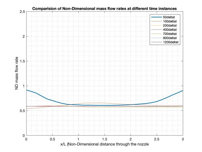
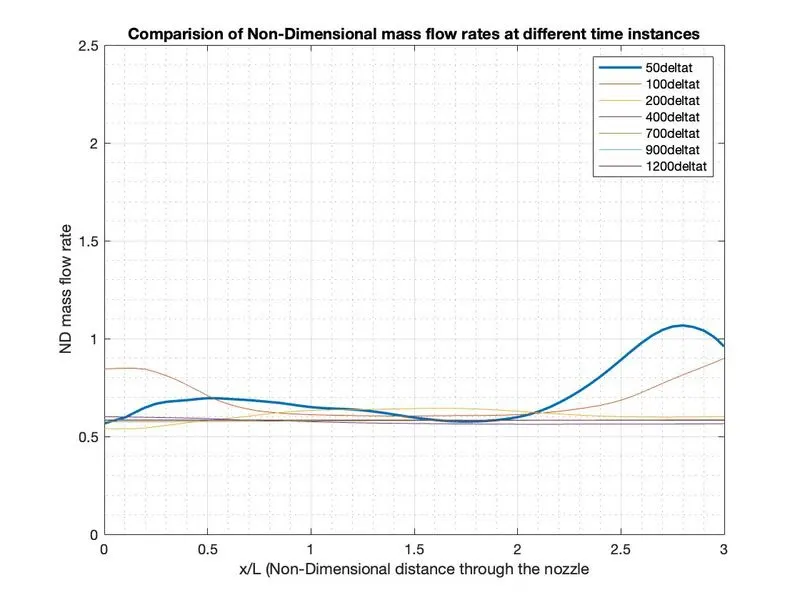
1. Non Conservative form:

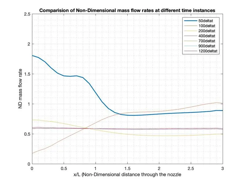
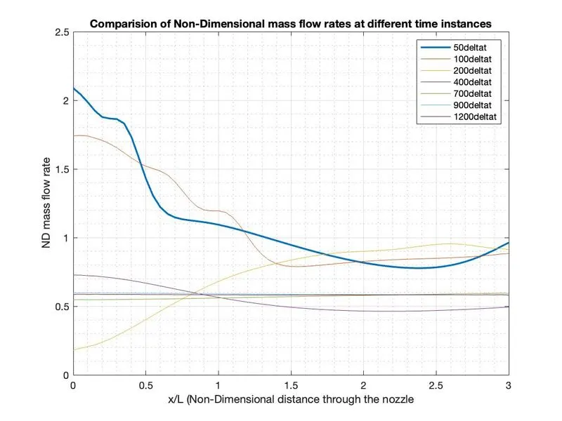
The Variation of mass flow rate at the nozzle at different time steps:(for N= 31 and N= 61 on left and right respectively)

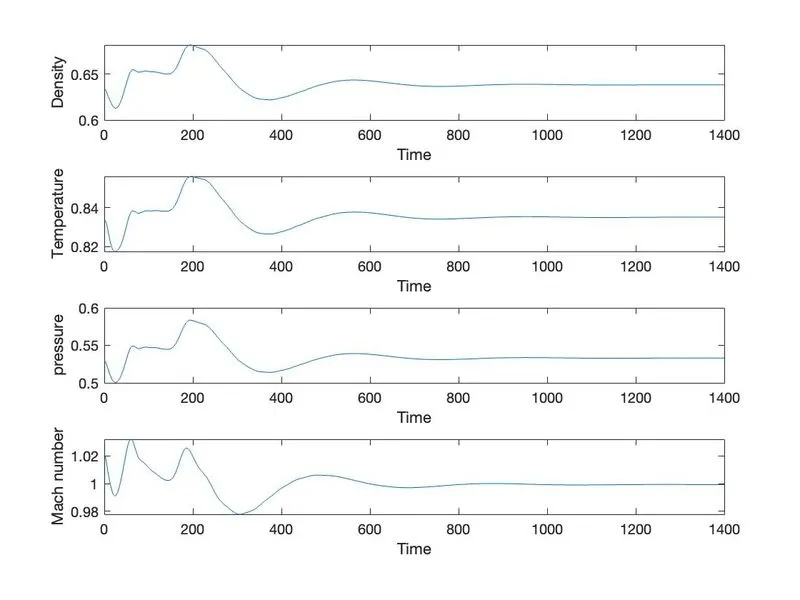
Variation of flow properties with respect to time(for N= 31 and N= 61 on left and right respectively)

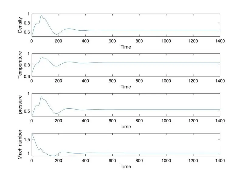
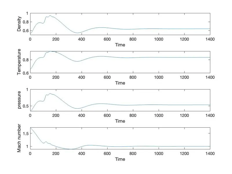
2.Conservative form:

variation of mass flow rate at the nozzle at different time steps(for N= 31 and N= 61 on left and right respectively)

Variation of flow properties with time (for N= 31 and N= 61 on left and right respectively)

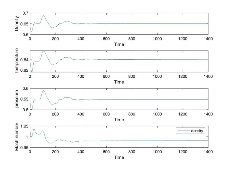
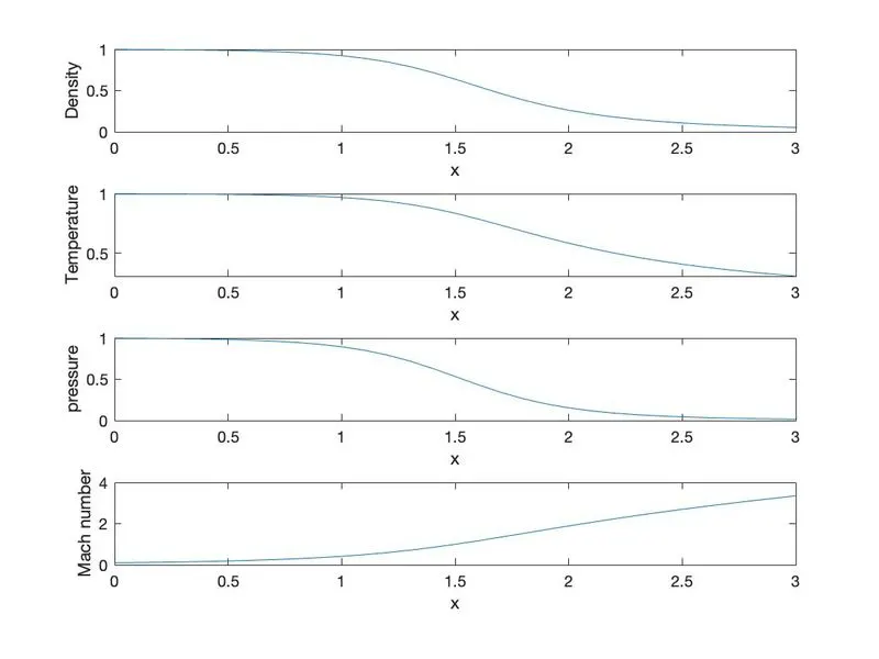
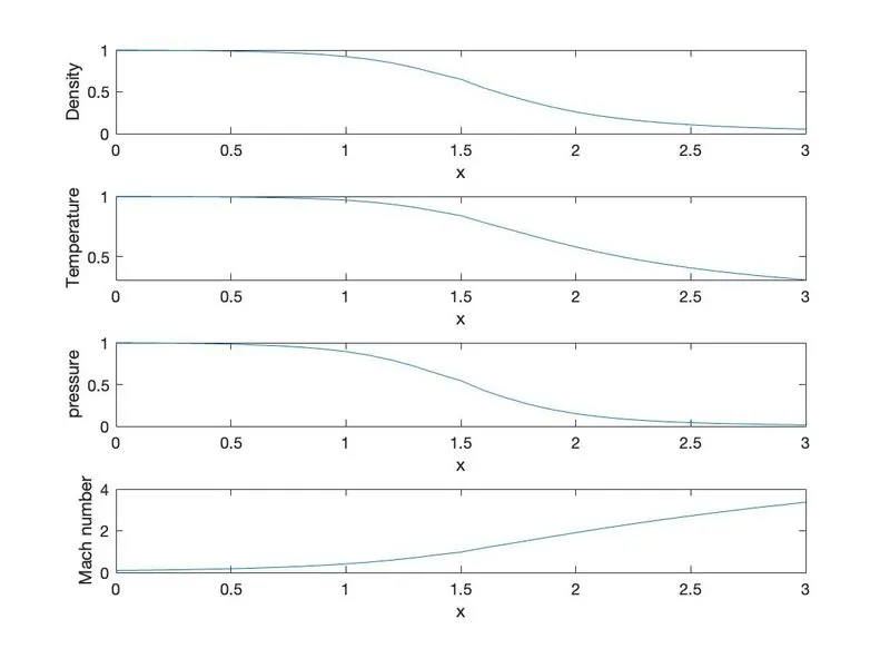
variation of flow properties along with x for Non conservative(on the left) and Conservative( on the right) forms

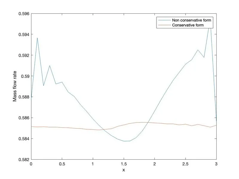
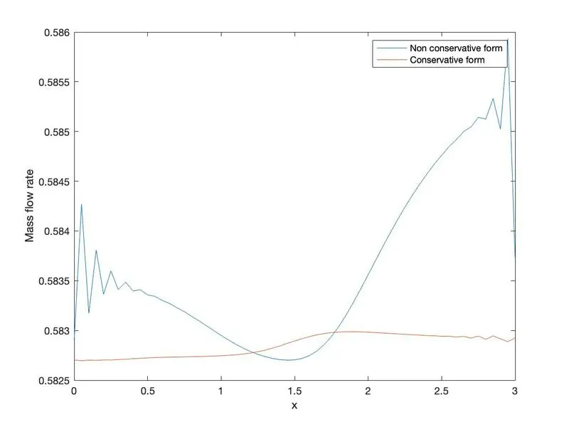
Mass flow rate Non conservative vs Conservative forms(for N= 31 and N= 61 on left and right respectively)

Grid Dependence test:

Computation time comparision and comparision of Flow properties at the throat of the nozzle in Non Conservative and conservative forms for N= 31 & N=61:

	Density`rho`	Temperature	Pressure Ratio	Mach Number	Computation time
Non conservative form at N= 31	0.6387	0.8365	0.5342	0.9994	0.862223
Conservative form at N= 31	0.6505	0.8401	0.5464	0.9817	0.478238
Non conservative form at N= 61	0.6377	0.8354	0.5327	0.9998	0.904732
Conservative form at N= 61	0.6383	0.8351	0.5331	0.9993	0.494727
Exact solution	0.638	0.835	0.533	0.997	-

Conclusion:

From the mass flow rate comparision graphs, we can infer that the Conservative form seems to be more stable than the Non conservative form.

The time taken and the minimum number og time steps required to attain stability via conservative form is comparitively lesser than that by Non conservative form. Thus making conservative form to be faster than Non conservative form.

From the grid dependence test, we see that the Non Conservative form is much closer to the Analytical solution on comparing with that of conservative form for both N=31 & N=61.

A grid dependence test is performed to see the effect of magnitide of theh number of grids has over the solution and we get to know from the above table on grid dependence, that as the number of grid iincreases the accuracy increases but the computation time increases.

Also a study on the effect of CFL on the solution was made and found that above C=1.11, the solution blew and became unstable, also when C is lesser than 0.2. C=0.5 showed comparitively stable solutions.

When it comes to flux quantities, the conservative form shows a more accurate solution, but Non conservative form shows comapritively more accurate solution for the primitive variables.

Apart from the above conclusions,the Non conservative form can only be a choice for numerical methods, if they dont have any sort of discontinuity in the solution. While, Conservative form, by definition, considers such discontuinties. With all that said, Consrvative form is comparitively the most preferred.