Week 11 - Simulation of Flow through a pipe in OpenFoam

Objective :

• To simulate the Hagon-Poiseuille flow through a pipe in OpenFOAM
• To write a MATLAB code to automate the generation of the computational mesh for any chosen wedge angle(i.e., is less than 5 degrees) and grading schemes.
• To show that the velocity profile of a baseline mesh matches with the Hagen Poiseuille Equation.
• To validate the fully developed velocity profile and post process shear stress developed using Paraview.

Methodology:

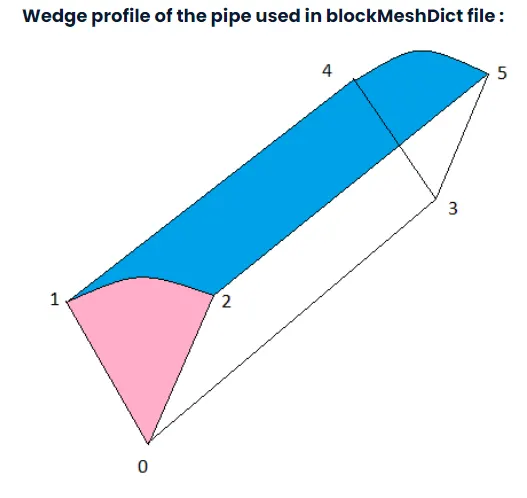
As mentioned our objective is to simulate the Hagen-Poiseuille flow through a pipe of circular cross section, with all the assumptions made. With the flow being axissymmetric in nature(i.e., symmetric along the axis of the cylindrical pipe), we reduce the model into a wedge, thus modelling only a section of a cylindrical pipe through which the fluid flow will be simulated, reducing the complexity of the problem and also the computational resources required, in a more efficeint way. The wedge is created by considering a specific wedge angle which shall be less than 5 degrees. A MATLAB script is created to auto-generate the computational mesh with the wedge angle as the input. The output from this script will be used as the blockMeshDict file. The icoFoam solver(used to solve incompressible,laminar,Navier-stokes equation) is used to simulate the flow through the pipe. The results are then post-processed using ParaView, to observe and validate the velocity profile for the fully developed flow, and at the hydrodynamic entrance length of the pipe. The variation of Shear stress developed across the radius of the pipe along length of the pipe is also plotted and all these simulations are validated by comparing with the analytical solutions obtained from the Hagen-Poiseuille equations ensuring the validity of the results.

Hagen-Poiseuille flow:

The Hagen-Poiseuille flow is a type of fluid flow based on the Hagen-Poiseuille Law, which is a physical law that gives the pressure drop in an incompressible and Newtonian fluid in laminar flow flowing through a long cylindrical pipe of constant cross-section. Hagen-Poiseuille flow is the guiding principle behind a variety of applications like, air flow through the lung alveoli, fluid flow through a drinking straw or through a hypodermic needle. In essence, Poiseuille's equation is used to describe the pressure drop caused by the viscosity of the fluid.

The assumptions of the HP equation is that,

• the fluid is incompressible and Newtonian
• the flow is laminar through a pipe of constant cross section, with a length that is sufficiently larger than the diameter of the pipe
• there is no acceleration of the fluid through the pipe

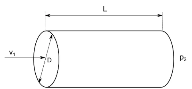
Consider a cylindrical pipe of circular cross section as shown above. Let the diameter of the pipe be D and the Length of the pipe be 'L'. Assume a fluid flowing through this pipe with an inlet velocity of `v_1` and let pressure at the outlet of the pipe be `p_2`. Let's assume the diameter of the pipe to be 0.02 m, i.e., 20 mm. The length of the pipe will be decided based on the Hydrodynamic entrance Length (L_e) obtained, which will be explained in upcoming sections. Let water be the working fluid flowing through the pipe. Since, Hagen-Poiseuille flow is a laminar flow, a Reynold's Number pertaining to laminar flow regime (Re=2100) is considered to simulate the fluid flow and calculate the fluid velocity. In order to minimise the compuattional resources required for simulating the problem. a section of the pipe or a wedge with a specific wedge angle (less than 5 degrees) is considered, and the symmetry boundary conditions are applied. With all these assumed input values, a MATLAB script is created to automate the generation of the computational mesh and create the blockMeshDict file to be used in OpenFOAM`

Input parameters:

Diameter of the pipe (D)= 0.02 m

Wedge Angle (`Theta`)= 3 degrees

Density of the fluid (water) (`rho`) = 997 `(kg)/(m^3)`

Viscosity of the fluid (water) (`mu`) = `8.9e-4 Pa.s`at 298k

Reynold's Number for Laminar flow (Re) = 2100

Theory:

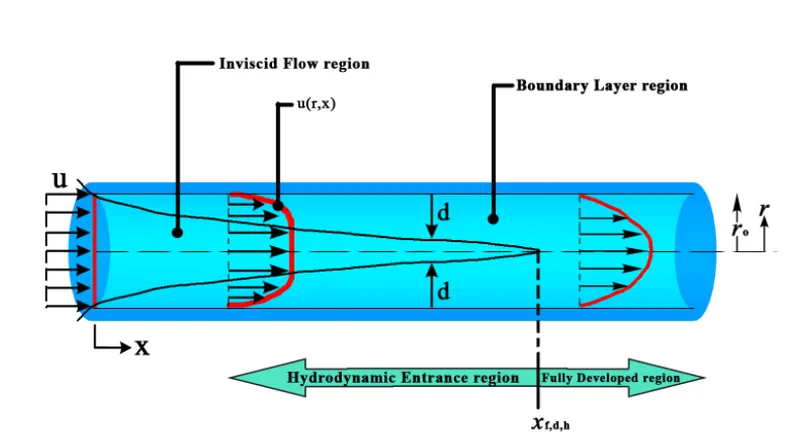
As the working fluid (water in our case) enters the pipe with a constant inlet velocity, the fluid comes in contact with the pipe walls. Because of the no-slip boundary condition, the fluid particles in the layer in contact with the wall come to a complete cease. This layer also causes the fluid particles in the adjacent layers to slow down gradually due to the friction between the layers which is nothing but the fluid viscosity. To make up for this velocity reduction, the velocity of the fluid at the mid section of the pipe has to increase so that the mass flow rate through the pipe remains constant. As a result of this, a velocity gradient develops along the axial direction of length of the pipe.

The region of flow in which the effects of viscous shearing forces caused by the fluid viscosity are significantly felt is called the velocity boundary layer. The boundary surface divides the flow in a pipe into two regions: The Boundary Layer region- where the viscous effects and velocity changes are significant, and The Inviscid flow region- where the friction effects are negligible and the velocity essentially remains constant in the radial direction. The thickness of the boundary layer gradually increases in the flow direction, until it reaches the mid-section of the pipe =, at which point it fills the entire pipe, and the velocity profile becomes fully developed. The region of the pipe from the pipe inlet, to the point at which the flow becomes fully developed is called as the hydrodynamic entrance region, and the length of this region is called the hydrodynamic entrance length (`L_e`). The flow in this region is called hydrodynamically developing flow since this is the region where the velocity profile develops and keeps changing. The region beyond the entrance region in which the velocity profile is fully developed and remains unchanged across the length of the pipe, is called the hydrodynamically fully developed region. The velocity profile in the fully developed region is Parabolic for laminar. For Laminar flow, the expression for calculating the hydrodynamic entrance length is given as follows,

`L_e`=0.06*Re*D`

We know that for Newtonian fluids, the shear stress is directly proportional to the velocity gradient. Thus,the shear stress at the pipe wall (`tau_w`) is also related to the slope of the velocity profile. Since the velocity profile remains unchanged in the fully developed region, the wall shear stress also remains constant in this region. Also, the wall sear stress is highest at the inlet where the thickness of the boundary layer is the smallest, and decreases gradually to the fully developed value. Other commonly used forms of the equation are described below.

`trianglep=(8muLV_(avg))/(R^2) and trianglep=(32muLV_(avg))/D^2`

where, `trianglep=p_1 -p_2`difference in pressure between the inlet and outlet of the pipe, and all the other quantities are as described earlier. From the above equation, it is clear that the pressure drop across the pipe is directly proportional to the viscosity of the fluid flowing through the pipe. Tf there were no viscosity(i.e. no friction), the pressure loss would be zero. Hence, the pressure drop in the above case is entirely due to the fluid viscosity.

Deriving Analytical solutions for flow parameters from Hagen-Poisiuelle equation:

1. Reynold's Number, Re=`(rhoV_(avg)D)/mu``implies`2100=`(997timesV_(avg)times0.02)/(8.92e-4)`

`V_(avg)`=0.0939m/s

2.Maximum Velocity at center line,`v_(max)=2.V_(avg)=0.1878`m/s

3. Maximum velocity entrance length

`L_h=0.06timesDtimesRe=0.06times0.02times2100=2.52m`

4. Pressure drop across the pipe from HP equation:

`trianglep=(32muLV_(avg))/(D^2)=(32times8.9e-4times3times0.0937)/(0.02^2)=18.89Pa`

5. Kinematic pressure drop= `(trianglep)/rho`=`20.012/997=0.0189Pa`

6.Velocity Profile at any location in fully developed region is given by

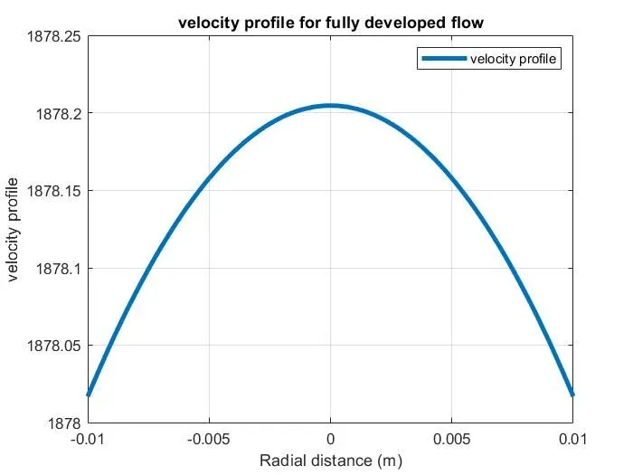
`U(r)=2.V(avg).(1-(r^2)/(R^2))`, where 'r' represents the radial distance from the centre of the pipe.

The Analytical values and equations described above will be used for comparing against the CFD results obtained to ensure their validity.

MATLAB code:

The MATLAB script file is written by assuming initial values for flow parameters as described earlier. The code is used to automatically generate the computational mesh, considering a specific wedge angle for the pipe.

clear all
close all
clc

%inputs
Re=2100; %Reynold Number
D=0.02; %Diameter of the pipe(in metres)
L_en=0.06*D*Re %hydrodynamic length at the enterance
L=L_en+0.3 %Total length of the pipe
R=D/2; %Radius of pipe in m
Rho= 997; %Density of water in kg/m^3
mu= 8.917e-4; %Kinematic viscoity of water in Pa.s
nu =mu/Rho
theta= 3;%wedge angle is an assumed that is less than 5 degrees

%Hagen-Poiseuille Equation:
V_avg=mu*Re/(Rho*D)
V_max=2*V_avg
delta_p=8*mu*V_avg*L/(R^2) %Pressure drop in Pa
Kinematic_p=delta_p/Rho %Kinematic pressure in m^2/s^2

%Analytical calculations of shear stress and velocity profile
r=linspace(-0.01,0.01,100);
for i=1:length(r)
    tau(i)=(2*mu*V_max*abs (r(i)))/(R^2);
    U(i)=V_max*(abs(1-(r(i).^2))/R^2);
end
figure(1)
plot(r,tau,'linewidth',3)
grid on
xlabel('Radial distance (m)')
ylabel('shear stress in N/m^2')
title('shear stress for fully developed flow')
legend('shear stress')
figure(2)
plot(r,U,"LineWidth",3)
grid on
xlabel('Radial distance (m)')
ylabel('velocity profile')
title('velocity profile for fully developed flow')
legend('velocity profile')

%Mesh
grading=0.2;
%grade_z=1;
b1=50;b2=1;b3=200;

%vertices of the wedge.
v0=[0 0 0]
v1=[0 R*cosd(theta/2) -R*sind(theta/2)]
v2=[0 R*cosd(theta/2) R*sind(theta/2)]
v3=[L 0 0]
v4=[L R*cosd(theta/2) -R*sind(theta/2)]
v5=[L R*cosd(theta/2) R*sind(theta/2)]

%creating blockMeshDict file
h1='/*------------------------------*- C++ -*-----------------------------*\';
h2='| =========                |                                           |';
h3='| \\      /  F ield        | OpenFOAM: The Open Source CFD Toolbox     |';
h4='|  \\    /   O peration    | Version:  4.1                             |';
h5='|   \\  /    A nd          | Web:      www.OpenFOAM.org                |';
h6='|    \\/     M anipulation |                                           |';
h7='\*--------------------------------------------------------------------*/';

h8='//********************************************************************//';

f1=fopen('blockMeshDict','w');

fprintf(f1,'%s\n',h1);
fprintf(f1,'%s\n',h2);
fprintf(f1,'%s\n',h3);
fprintf(f1,'%s\n',h4);
fprintf(f1,'%s\n',h5);
fprintf(f1,'%s\n',h6);
fprintf(f1,'%s\n \n',h7);

fprintf(f1,'FoamFile \n {\n')
fprintf(f1,'%16s %10s\n','version','2.0;')
fprintf(f1,'%16s %12s\n','format','ascii;')
fprintf(f1,'%16s %17s\n','class','dictionary;')
fprintf(f1,'%16s %20s\n','object','blockMeshDict;')
fprintf(f1,'%2s\n','}')

fprintf(f1,'%2s\n\n',h8);
fprintf(f1,'%2s\n\n','convertToMeters 1;')
fprintf(f1,'vertices\n(\n')
fprintf(f1,'    (%d %d %d)\n',v0)
fprintf(f1,'    (%d %d %d)\n',v1)
fprintf(f1,'    (%d %d %d)\n',v2)
fprintf(f1,'    (%d %d %d)\n',v3)
fprintf(f1,'    (%d %d %d)\n',v4)
fprintf(f1,'    (%d %d %d)\n',v5)
fprintf(f1,'%2s\n\n',');');

fprintf(f1,'blocks \n(\n')
fprintf(f1,'\t %s (%d %d %d) %s (1 1 1) \n','hex (0 1 2 0 3 4 5 3)',b1,b2,b3,'simpleGrading')
fprintf(f1,');\n\n')

fprintf(f1,'edges \n(\n')
fprintf(f1,'\t %s (0 %d 0)\n','arc 1 2',R)
fprintf(f1,'\t %s (%d %d 0)\n','arc 4 5',L,R)
fprintf(f1,'%2s\n\n',');')

fprintf(f1,'boundary \n(\n')
fprintf(f1,'\t %5s \n','axis','{')
fprintf(f1,'\t %13s %s\n','type','empty;')
fprintf(f1,'\t %14s\n %18s\n','faces','(')
fprintf(f1,'\t %15s\n %19s\n\n%14s\n\n','(0 3 3 0)',');','}')

fprintf(f1,'\t %5s \n','wall','{')
fprintf(f1,'\t %13s %s\n','type','wall;')
fprintf(f1,'\t %14s\n %18s\n','faces','(')
fprintf(f1,'\t\t %15s\n %19s \n\n %14s\n\n','(2 1 4 5)',');','}')

fprintf(f1,'\t %5s \n','inlet','{')
fprintf(f1,'\t %13s %s\n','type','patch;')
fprintf(f1,'\t %14s\n %18s\n','faces','(')
fprintf(f1,'\t\t %15s\n %19s \n\n %14s\n\n','(0 1 2 0)',');','}')

fprintf(f1,'\t %5s \n','outlet','{')
fprintf(f1,'\t %13s %s\n','type','patch;')
fprintf(f1,'\t %14s\n %18s\n','faces','(')
fprintf(f1,'\t\t %15s\n %19s \n\n %14s\n\n','(3 5 4 3)',');','}')

fprintf(f1,'\t %5s \n','wedgeFront','{')
fprintf(f1,'\t %13s %s\n','type','wedge;')
fprintf(f1,'\t %14s\n %18s\n','faces','(')
fprintf(f1,'\t\t %15s\n %19s \n\n %14s\n\n','(1 0 3 4)',');','}')

fprintf(f1,'\t %5s \n','wedgeBack','{')
fprintf(f1,'\t %13s %s\n','type','wedge;')
fprintf(f1,'\t %14s\n %18s\n','faces','(')
fprintf(f1,'\t\t %15s\n %19s \n\n %14s\n\n','(2 5 3 0)',');','}')
fprintf(f1,');\n\n')

fprintf(f1,'mergePatchPairs \n (\n);\n')
fprintf(f1,'%2s\n\n',h8)

fclose(f1);

blockMeshDict file:

/*------------------------------*- C++ -*-----------------------------*\
| =========                |                                           |
| \\      /  F ield        | OpenFOAM: The Open Source CFD Toolbox     |
|  \\    /   O peration    | Version:  4.1                             |
|   \\  /    A nd          | Web:      www.OpenFOAM.org                |
|    \\/     M anipulation |                                           |
\*--------------------------------------------------------------------*/
 
FoamFile 
 {
         version       2.0;
          format       ascii;
           class       dictionary;
          object       blockMeshDict;
 }
//********************************************************************//

convertToMeters 1;

vertices
(
    (0 0 0)
    (0 9.996573e-03 -2.617695e-04)
    (0 9.996573e-03 2.617695e-04)
    (2.820000e+00 0 0)
    (2.820000e+00 9.996573e-03 -2.617695e-04)
    (2.820000e+00 9.996573e-03 2.617695e-04)
);

blocks 
(
	 hex (0 1 2 0 3 4 5 3) (50 1 200) simpleGrading (1 1 1) 
);

edges 
(
	 arc 1 2 (0 1.000000e-02 0)
	 arc 4 5 (2.820000e+00 1.000000e-02 0)
);

boundary 
(
	  axis 
	     { 
	          type empty;
	          faces
                  (
	       (0 3 3 0)
                  );

             }

	  wall 
	     { 
	          type wall;
	          faces
                  (
		       (2 1 4 5)
                  ); 

              }

	 inlet 
	     { 
	          type patch;
	          faces
                  (
		       (0 1 2 0)
                  ); 

              }

	 outlet 
	     { 
	          type patch;
	          faces
                  (
		       (3 5 4 3)
                  ); 

              }

	 wedgeFront 
	     { 
	          type wedge;
	          faces
                  (
		       (1 0 3 4)
                  ); 

              }

	 wedgeBack 
	     { 
	          type wedge;
	          faces
                  (
		       (2 5 3 0)
                  ); 

              }

);

mergePatchPairs 
(
);
//********************************************************************//

controlDict file:

/*--------------------------------*- C++ -*----------------------------------*\
  =========                 |
  \\      /  F ield         | OpenFOAM: The Open Source CFD Toolbox
   \\    /   O peration     | Website:  https://openfoam.org
    \\  /    A nd           | Version:  9
     \\/     M anipulation  |
\*---------------------------------------------------------------------------*/
FoamFile
{
    format      ascii;
    class       dictionary;
    location    "system";
    object      controlDict;
}
// * * * * * * * * * * * * * * * * * * * * * * * * * * * * * * * * * * * * * //

application     icoFoam;

startFrom       startTime;

startTime       0;

stopAt          endTime;

endTime         5;

deltaT          0.01;

writeControl    timeStep;

writeInterval   100;

purgeWrite      0;

writeFormat     ascii;

writePrecision  6;

writeCompression off;

timeFormat      general;

timePrecision   6;

runTimeModifiable true;


// ************************************************************************* //

transportProperties file:

/*--------------------------------*- C++ -*----------------------------------*\
  =========                 |
  \\      /  F ield         | OpenFOAM: The Open Source CFD Toolbox
   \\    /   O peration     | Website:  https://openfoam.org
    \\  /    A nd           | Version:  9
     \\/     M anipulation  |
\*---------------------------------------------------------------------------*/
FoamFile
{
    format      ascii;
    class       dictionary;
    location    "constant";
    object      transportProperties;
}
// * * * * * * * * * * * * * * * * * * * * * * * * * * * * * * * * * * * * * //

nu              [0 2 -1 0 0 0 0] 8.9438e-07;


// ************************************************************************* //

velocity file

/*--------------------------------*- C++ -*----------------------------------*\
  =========                 |
  \\      /  F ield         | OpenFOAM: The Open Source CFD Toolbox
   \\    /   O peration     | Website:  https://openfoam.org
    \\  /    A nd           | Version:  9
     \\/     M anipulation  |
\*---------------------------------------------------------------------------*/
FoamFile
{
    format      ascii;
    class       volVectorField;
    object      U;
}
// * * * * * * * * * * * * * * * * * * * * * * * * * * * * * * * * * * * * * //

dimensions      [0 1 -1 0 0 0 0];

internalField   uniform (0.0939 0 0);

boundaryField
{
    axis
    {
        type            empty;
    }
   
    inlet
    {
        type            fixedValue;
        value           uniform (0.0939 0 0);
    }

   outlet
   {
       type             zeroGradient;
   }

    wall
    {
        type            noSlip;
    }

    wedgeFront
    {
        type            wedge;
    }

    wedgeBack
    {
        type            wedge;
    }
}

// ************************************************************************* //

pressure file:

/*--------------------------------*- C++ -*----------------------------------*\
  =========                 |
  \\      /  F ield         | OpenFOAM: The Open Source CFD Toolbox
   \\    /   O peration     | Website:  https://openfoam.org
    \\  /    A nd           | Version:  9
     \\/     M anipulation  |
\*---------------------------------------------------------------------------*/
FoamFile
{
    format      ascii;
    class       volScalarField;
    object      p;
}
// * * * * * * * * * * * * * * * * * * * * * * * * * * * * * * * * * * * * * //

dimensions      [0 2 -2 0 0 0 0];

internalField   uniform 0;

boundaryField
{
    axis
    {
        type            empty;
    }

    inlet
    {
        type            zeroGradient;
    } 

    wall
    {
        type            zeroGradient;
    } 

    wedgeFront
    {
        type            wedge;
    }

    wedgeBack
    {
        type            wedge;
    }

    outlet
    {
        type            fixedValue;
        value           uniform 0;
    }

}

// ************************************************************************* //

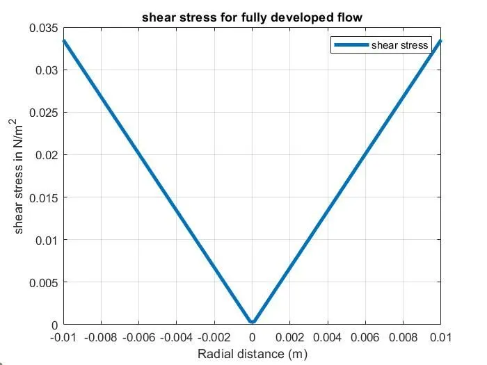
Analytical Results from MATLAB :

Computational Results from OpenFOAM:

Mesh information:

no.of Points: 20301

no. of Cells: 10000

no. of Faces: 40050

no. of InternalFaces: 19750

Courant Number mean: 0.0684214

Courant Number max: 0.219637

Time Taken : 55s

Computational Results from Paraview:

The animation of the variation of pressure and velocity across the pipe are being attached below.

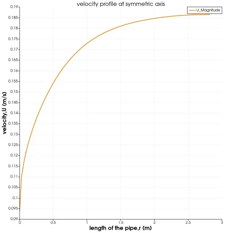
Variation of pressure and velocity along the symmetric axis, i.e, center of the pipe:

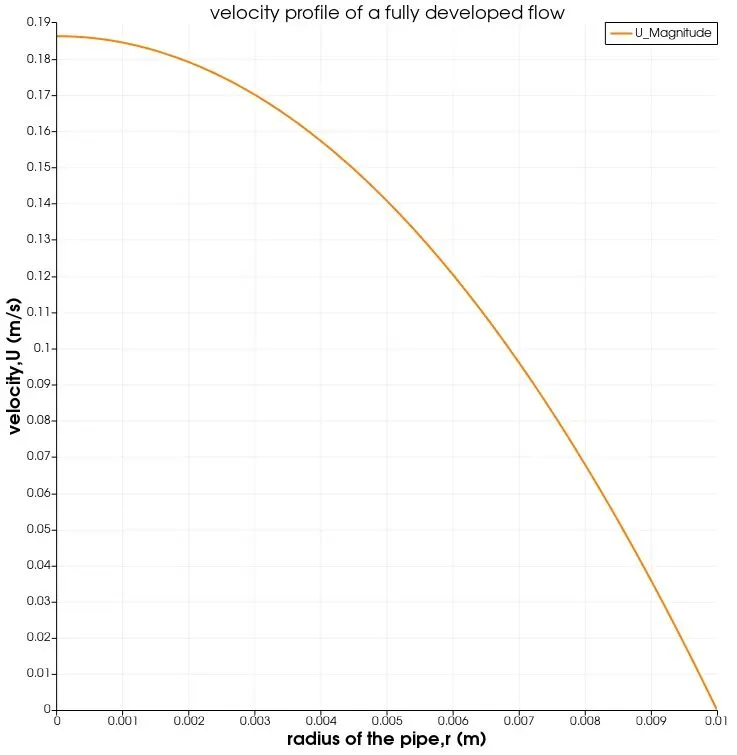
Variation of the pressure and velocity at x= 2.53 m (fully developed flow)

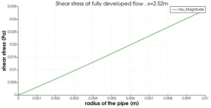
Shear stress at fully developed flow,x=2.53* m:

Conclusion:

1. Hydrodynamic Length:

From the computed graphs via paraview, we get that after x=2.53 mm, the velocity is being almost constant, thus the computed hydrodynamic entrance length should be around 2.53 m according to the simulation, while the analytical value of the hydrodynamic entrance length is 2.52 m, thus having minimal error.

2. Velocity Profile:

The Theoritical Velocity profile at a fully developed flow region(x=2.52 m) is almost similar to the computed velocity profile at a fully developed flow region (x=2.53 m). Across the length of the pipe, the variation in velocity, in the computed velocity profile, till somewhere around x=2.53 m indicates the effect of viscosity till it reaches the hydrodynamic entrance length.

3. Maximum velocity:

The theoretical value of the maximum velocity was 0.187 m/s, while the computed value of the same is 0.186 m/s, thus having a minimal error.

4. shear stress:

At the start of the pipe , there is a small part where the shear stress is not linear,which explains the no slip condition, but as the length increases,the shear stress becomes linear, thus explaining nature of developed flow

contours:

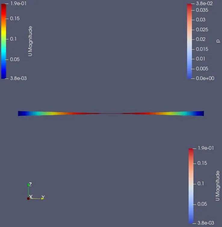
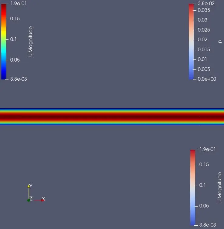
Animations of velocity profile along the symmetric axis and shear stress and velocity profile at fully developed flow region are attached below respectively.