Week 5.1 - Mid term project - Solving the steady and unsteady 2D heat conduction problem
Solving Steady and unsteady 2D heat conduction equation
Aim:
To compute and compare the solutions and errors from the different point-iterative solving techniques such as Jacobi, Gauss-Seidel & Successive over relaxation method for the implicit scheme of differencing for both Transient and steady states of 2D heat conduction equation.
Theory:
The Steady state 2D heat conduction equation is given by
`(del^2T)/(delx^2)+(del^2T)/(dely^2)=0`
Discretizing and simplifying the above equation using central differencing scheme gives us
`T_p=(1/k)((T_L+T_R)/(triangle x)^2 +(T_T+T_B)/(triangley)^2)`
where, k =`((trianglex)^2+(triangley)^2)/((trianglex)^2*(triangley)^2)`
also ,`T_L=T_(i-1,j)`;`T_R=T_(i+1,j)`;`T_T=T_(i,j+1)`;`T_B=T_(i,j-1)`
Jacobi method:
`(T_(p+1))^(n+1)=(1/k)((T_L+T_R)/(triangle x)^2 +(T_T+T_B)/(triangley)^2)^n`
Gauss-Seidel method:
`(T_(p+1))^(n+1)=(1/k)((T_L+T_R)/(triangle x)^2 +(T_T+T_B)/(triangley)^2)^(n+1)`
Successive over relaxation method:
`(T_(p+1))^(n+1)=(T_p)^(n) (1-omega)+ omega(1/k)((T_L+T_R)/(triangle x)^2 +(T_T+T_B)/(triangley)^2)^(n+1)`
The Transient state 2D heat conduction equation is given by
`(delT)/(delt)=alpha((del^2T)/(delx^2)+(del^2T)/(dely^2))`
Discretizing and simplifying the above equation using forward differencing scheme for time derivative and central differencing scheme for space derivative gives us
For explicit scheme:
`(T_p)^(n+1)=(T_p)^n (1-2k_1 -2k_2)+[k_1(T_L+T_R) + k_2(T_T+T_B)]^(n+1)`
where,
`CFL_x=k_1=alpha(trianglet)/(trianglex)^2`
`CFL_y=k_2=alpha(trianglet)/(triangley)^2`
The CFL stability condition for this explicit diffusion problem in 2D is given by
`CFL_x+CFL_y<=0.5`
For Implicit scheme:
`(T_p)^(n+1)=a(T_p)^n +[b(T_L+T_R) + c(T_T+T_B)]^(n+1)`
where
`a= 1/(1-2k_1 -2k_2)`;`b=ak_1`;`c=ak_2`
Jacobi method
`(T_p)^(n+1)=a(T_p)^n +[b(T_L+T_R) + c(T_T+T_B)]^(n)`
Gauss-Seidel method:
`(T_p)^(n+1)=a(T_p)^n +[b(T_L+T_R) + c(T_T+T_B)]^(n+1)`
Successive over relaxation method:
`(T_p)^(n+1)=(T_p)^(n+1) (1-omega) +omega (a(T_p)^n +[b(T_L+T_R) + c(T_T+T_B)])^(n+1)`
Inputs:
A square of side 1m was assumed as the domain.
No. of node points at x and y directions are taken as `n_x=n_y=21`
Boundary conditions:
Assumed initial temperature of the domain = 298k
T at top boundary=600k,
T at bottom boundary =900k
T at left boundary = 400k
T at right boundary = 800k
T at Top left corner = 500k
T at Top right corner = 700k
T at bottom left corner = 650k
T at bottom right corner = 850k
Error tolerence = 1e-4
Matlab code:
main script:
clear all
close all
clc

Jacobi_SS();%Jacobi method for analysis of Steady state of 2D heat coduction equation
GS_SS();%Gauss-Seidel method for analysis of Steady state of 2D heat coduction equation
SOR_SS();%SOR method for analysis of Steady state of 2D heat coduction equation
Jacobi_ITS();%Jacobi method for analysis of transient state of 2D heat coduction equation
GS_ITS();%Gauss-Seidel method for analysis of transient state of 2D heat coduction equation
SOR_ITS();%SOR method for analysis of transient state of 2D heat coduction equation
ETS();%Analysis of transient state of 2D heat coduction equation using explicit scheme
function codes:
Jacobi for Steady state :
function Jacobi_SS()

nx=21;ny=21; %mesh
T=298*ones(nx,ny);%assumed initial condition
%BC
T(:,1)=400;%left
T(:,ny)=800;%right
T(nx,:)=900;%Bottom
T(1,:)=600;%Top
T(1,1)=500;%left-top
T(nx,1)=650;%left-bottom
T(1,ny)=700;%right-top
T(nx,ny)=850;%right-bottom


T_old=T;
x=linspace(0,1,nx); dx=x(2)-x(1);
y=linspace(0,1,ny); dy=y(2)-y(1);
[X,Y]=meshgrid(x,y);
tol=1e-4; %error tolerance
error=1;
k=2*((dx^2)+(dy^2))/((dx^2)*(dy^2));
n_iter=1;
    tic
    while(error>tol)
        for i=2:nx-1
            for j= 2:ny-1
                T(i,j)=(1/k)*((T_old(i-1,j)+T_old(i+1,j))/(dx^2)+(T_old(i,j-1)+T_old(i,j+1))/(dy^2));
            end
        end
        error=max(max(abs(T_old-T)));
        T_old=T;
        n_iter=n_iter + 1;
    end
    figure(1)
    [l,h]=contourf(X,Y,T);
    clabel(l,h);
    xlabel('x'); ylabel('y');
    title('Jacobi method for Analysis of Steady State of 2D heat conduction equation');
    sim_time1=toc;
    subtitle(sprintf('Simulation time=%f',sim_time1));
    subtitle(sprintf('no. of iterations = %f',n_iter));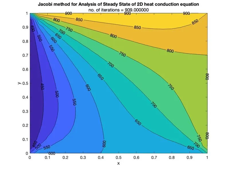
Gauss-Seidel for Steadt state:
function GS_SS()

nx=21;ny=21; %mesh
T=298*ones(nx,ny);%assumed initial condition
%BC
T(:,1)=400;%left
T(:,ny)=800;%right
T(nx,:)=900;%Bottom
T(1,:)=600;%Top
T(1,1)=500;%left-top
T(nx,1)=650;%left-bottom
T(1,ny)=700;%right-top
T(nx,ny)=850;%right-bottom


T_old=T;
x=linspace(0,1,nx); dx=x(2)-x(1);
y=linspace(0,1,ny); dy=y(2)-y(1);
[X,Y]=meshgrid(x,y);
tol=1e-4; %error tolerance
error=1;
k=2*((dx^2)+(dy^2))/((dx^2)*(dy^2));
n_iter=1;

    %Gauss-seidel method
    while(error>tol)
        for i=2:nx-1
            for j=2:ny-1
                T(i,j)=(1/k)*((T(i-1,j)+T(i+1,j))/(dx^2)+(T(i,j-1)+T(i,j+1))/(dy^2));
            end
        end
        error=max(max(abs(T_old-T)));
        T_old=T;
        n_iter=n_iter + 1;
    end
    figure(2)
    [l,h]=contourf(X,Y,T);
    clabel(l,h)
    xlabel('x'); ylabel('y');
    title('Analysis of Steady State of 2D heat conduction equation using Gauss-seidel method');
    sim_time2=toc;
    subtitle(sprintf('Simulation time=%f',sim_time2));
    subtitle(sprintf('no. of iterations = %f',n_iter));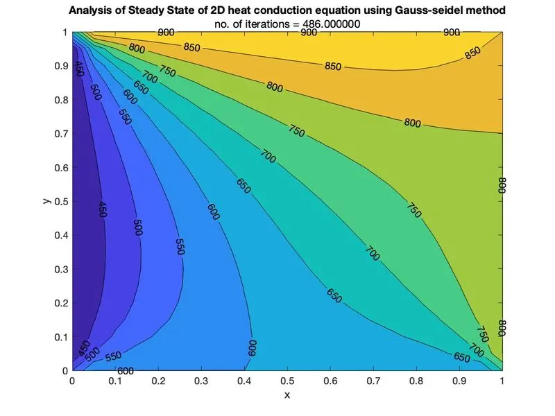
SOR for steady state:
function SOR_SS()

nx=21;ny=21; %mesh
T=298*ones(nx,ny);%assumed initial condition
%BC
T(:,1)=400;%left
T(:,ny)=800;%right
T(nx,:)=900;%Bottom
T(1,:)=600;%Top
T(1,1)=500;%left-top
T(nx,1)=650;%left-bottom
T(1,ny)=700;%right-top
T(nx,ny)=850;%right-bottom


T_old=T;
x=linspace(0,1,nx); dx=x(2)-x(1);
y=linspace(0,1,ny); dy=y(2)-y(1);
[X,Y]=meshgrid(x,y);
tol=1e-4; %error tolerance
error=1;
k=2*((dx^2)+(dy^2))/((dx^2)*(dy^2));
n_iter=1;

    tic
    %Successive ove relaxation method
    omega=1.5;
    while(error>tol)
        for i=2:nx-1
            for j=2:ny-1
                T(i,j)=(1-omega)*T(i,j)+(omega*(1/k)*((T(i-1,j)+T(i+1,j))/(dx^2)+(T(i,j-1)+T(i,j+1))/(dy^2)));
            end
        end
        error=max(max(abs(T_old-T)));
        T_old=T;
        n_iter=n_iter+1;
    end
    figure(3)
    [l,h]=contourf(X,Y,T);
    clabel(l,h)
    xlabel('x'); ylabel('y');
    title('SOR for Gauss-seidel method for analysis of Steady State of 2D heat conduction equation');
    sim_time3=toc;
    subtitle(sprintf('Simulation time=%f',sim_time3));
    subtitle(sprintf('no. of iterations = %f',n_iter));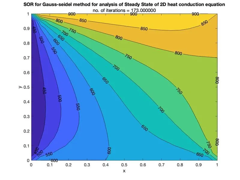
Explicit scheme for Transient state :
function ETS()

nx=21;ny=21; %mesh
T=298*ones(nx,ny);%assumed initial condition
%BC
T(:,1)=400;%left
T(:,ny)=800;%right
T(nx,:)=900;%Bottom
T(1,:)=600;%Top
T(1,1)=500;%left-top
T(nx,1)=650;%left-bottom
T(1,ny)=700;%right-top
T(nx,ny)=850;%right-bottom


T_old=T;
x=linspace(0,1,nx); dx=x(2)-x(1);
y=linspace(0,1,ny); dy=y(2)-y(1);
[X,Y]=meshgrid(x,y);
tol=1e-4; %error tolerance
error=1;
run_time=50;
dt=0.0002;%time step
nt=run_time/dt;
alpha=1.5;
k1=alpha*dt/(dx^2);
k2=alpha*dt/(dy^2);
n_iter=1;
CFL= k1+k2;


tic
%Explicit scheme of solving 2D heat conduction equation

for k=1:nt %time loop
    for i=2:nx-1
        for j=2:ny-1
            T(i,j)=T_old(i,j)*(1-2*k1-2*k2)+k1*(T_old(i-1,j)+T_old(i+1,j))+ k2*(T_old(i,j-1)+T_old(i,j+1));
        end
    end
    error=max(max(abs(T_old-T)));
    T_old=T;
    n_iter=n_iter+1;

end
  figure(4)
    [l,h]=contourf(X,Y,T);
    clabel(l,h)
    xlabel('x'); ylabel('y');
    title('Analysis of Transient State of 2D heat conduction equation using explicit method');
    sim_time4=toc;
    subtitle(sprintf('Simulation time=%f',sim_time4));
    subtitle(sprintf('no. of iterations = %f',n_iter));
 subtitle(sprintf('Error=%d',error));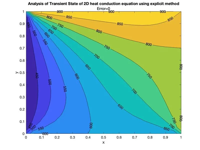
Jacobi method for transient state
function Jacobi_ITS()

nx=21;ny=21; %mesh
T=298*ones(nx,ny);%assumed initial condition
%BC
T(:,1)=400;%left
T(:,ny)=800;%right
T(nx,:)=900;%Bottom
T(1,:)=600;%Top
T(1,1)=500;%left-top
T(nx,1)=650;%left-bottom
T(1,ny)=700;%right-top
T(nx,ny)=850;%right-bottom


T_old=T; T_prev=T;
x=linspace(0,1,nx); dx=x(2)-x(1);
y=linspace(0,1,ny); dy=y(2)-y(1);
[X,Y]=meshgrid(x,y);
tol=1e-4; %error tolerance
error=1;
run_time=5;
dt=0.0002;%time step
nt=run_time/dt;
alpha=1.5;
k1=(alpha*dt)/(dx^2);
k2=(alpha*dt)/(dy^2);
n_iter=1;
a=1/(1+2*k1+2*k2);
b=a*k1;
c=a*k2;
CFL=k1+k2
tic
%Jacobi method for transient state analysis of 2D heat conduction equation
for k=1:nt
    error=1;
 while(error>tol)
     for i=2:nx-1
         for j=2:ny-1
             T(i,j)=a*T_prev(i,j)+b*(T_old(i-1,j)+T_old(i+1,j))+ c*(T_old(i,j-1)+T_old(i,j+1));
         end
     end
     error=max(max(abs(T_old-T)));
     T_old=T;
     n_iter=n_iter+1;
 end
 T_prev=T;
end

figure(5)
[l,h]=contourf(X,Y,T);
clabel(l,h)
xlabel('x'); ylabel('y');
title('Analysis of Transient State of 2D heat conduction equation using Jacobi method of implicit scheme');
sim_time5=toc;
subtitle(sprintf('Simulation time=%f',sim_time5));
subtitle(sprintf('no. of iterations = %f',n_iter));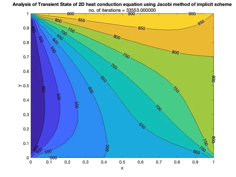
Gauss-Seidel for transient state:
function GS_ITS()

nx=21;ny=21; %mesh
T=298*ones(nx,ny);%assumed initial condition
%BC
T(:,1)=400;%left
T(:,ny)=800;%right
T(nx,:)=900;%Bottom
T(1,:)=600;%Top
T(1,1)=500;%left-top
T(nx,1)=650;%left-bottom
T(1,ny)=700;%right-top
T(nx,ny)=850;%right-bottom


T_old=T; T_prev=T;
x=linspace(0,1,nx); dx=x(2)-x(1);
y=linspace(0,1,ny); dy=y(2)-y(1);
[X,Y]=meshgrid(x,y);
tol=1e-4; %error tolerance
error=1;
run_time=5;
dt=0.0002;%time step
nt=run_time/dt;
alpha=1.5;
k1=alpha*dt/(dx^2);
k2=alpha*dt/(dy^2);
n_iter=1;
a=1/(1+2*k1+2*k2);
b=a*k1;
c=a*k2;
CFL=k1+k2
tic
%Gauss-seidel method for Transient state analysis of 2D heat conduction equation
for k=1:nt
    error=1;
 while(error>tol)
     for i=2:nx-1
         for j=2:ny-1
             T(i,j)=a*T_prev(i,j)+b*(T(i-1,j)+T(i+1,j))+ c*(T(i,j-1)+T(i,j+1));
         end
     end
     error=max(max(abs(T_old-T)));
     T_old=T;
     n_iter=n_iter+1;
 end
T_prev=T;
end

figure(6)
[l,h]=contourf(X,Y,T);
clabel(l,h)
xlabel('x'); ylabel('y');
title('Analysis of Transient State of 2D heat conduction equation using Gauss-seidel method of implicit scheme');
sim_time6=toc;
subtitle(sprintf('Simulation time=%f',sim_time6));
subtitle(sprintf('no. of iterations = %f',n_iter));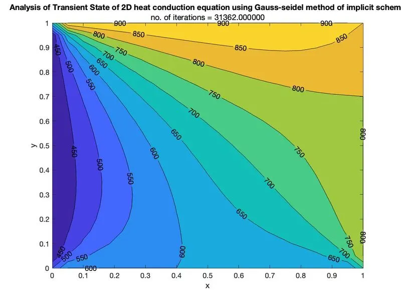
SOR for Transient method:
function SOR_ITS()

nx=21;ny=21; %mesh
T=298*ones(nx,ny);%assumed initial condition
%BC
T(:,1)=400;%left
T(:,ny)=800;%right
T(nx,:)=900;%Bottom
T(1,:)=600;%Top
T(1,1)=500;%left-top
T(nx,1)=650;%left-bottom
T(1,ny)=700;%right-top
T(nx,ny)=850;%right-bottom


T_old=T; T_prev=T;
x=linspace(0,1,nx); dx=x(2)-x(1);
y=linspace(0,1,ny); dy=y(2)-y(1);
[X,Y]=meshgrid(x,y);
tol=1e-4; %error tolerance
error=1;
run_time=5;
dt=0.0002;%time step
nt=run_time/dt;
alpha=1.5;
k1=alpha*dt/(dx^2);
k2=alpha*dt/(dy^2);
n_iter=1;
a=1/(1+2*k1+2*k2);
b=a*k1;
c=a*k2;
CFL=k1+k2
tic
for k=1:nt
%SOR of Gauss-seidel method for Transient state analysis of 2D heat conduction equation
omega=1.2;
error=1;
while(error>tol)
     for i=2:nx-1
         for j=2:ny-1
             T(i,j)=(1-omega)*T_old(i,j)+omega*(a*T_prev(i,j)+b*(T(i-1,j)+T(i+1,j))+ c*(T(i,j-1)+T(i,j+1)));
         end
     end
     error=max(max(abs(T_old-T)));
     T_old=T;
     n_iter=n_iter+1;
end
T_prev=T;
end

figure(7)
[l,h]=contourf(X,Y,T);
clabel(l,h)
xlabel('x'); ylabel('y');
title('SOR of Gauss-seidel method for analysis of Transient State of 2D heat conduction equation');
sim_time7=toc;
subtitle(sprintf('Simulation time=%f',sim_time7));
subtitle(sprintf('no. of iterations = %f',n_iter));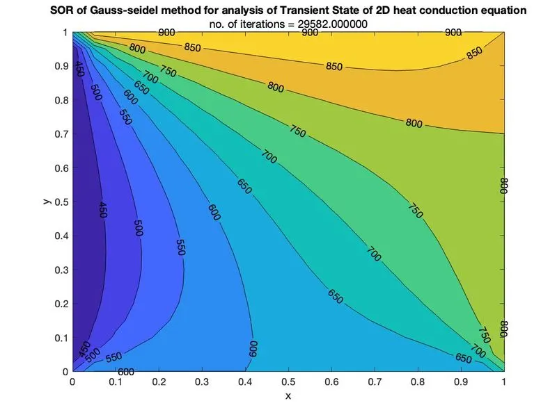
Observations:
| Method | No. of iterations | error |
| Jacobi for Steady state | 909 | 9.8235e-05 |
| Gauss-Seidel for steady state | 486 |
9.8391e-05 |
| SOR for Steady state | 173 | 9.6222e-05 |
| jacobi for transient state | 33553 | 0 |
| Gauss-Seidel for Transient state | 31362 | 0 |
| SOR for transient state | 29582 | 0 |
| Explicit scheme for transient | 250001 | 0 |
order of method based on iteration for both steady and unsteady cased
Jacobi>Gauss-Seidel>SOR, i.e., Jacobi takes more number of iterations to compute.