Week 9 - FVM Literature Review

Finite Volume Method

The finite volume method is a method for representing and evaluating partial diffrential equations in the form of algebraic equations.In the finite volume method, volume integrals in a partial differential equation that contain a divergence term are converted to surface integrals using the divergence thoerum . These terms are then evaluated as fluxes at the surfaces of each finite volume. Because the flux entering a given volume is identical to that leaving the adjacent volume, these methods are conservative Another advantage of the finite volume method is that it is easily formulated to allow for unstructured meshes. The method is used in many computational fluid dynamics packages. "Finite volume" refers to the small volume surrounding each node point on a mesh.

Finite volume methods can be compared and contrasted with the finite diffrence methods, which approximate derivatives using nodal values, or finite element methods, which create local approximations of a solution using local data, and construct a global approximation by stitching them together. In contrast a finite volume method evaluates exact expressions for the average value of the solution over some volume, and uses this data to construct approximations of the solution within cells.

Diffrence Between FDM and FVM

• Each method is quite similar in that it represents a systematic numerical method for solving PDEs.
• One important difference is the ease of implementation.
• A common opinion is that the finite-difference method is the easiest to implement and the finite-element method the most difficult.
• One reason for this may be that the finite-element method requires quite sophisticated mathematics for its formulation.

FDM Advantages and Disadvantages

The finite-difference method is defined dimension per dimension. this makes it easy to increase the “element order” to get higher-order accuracy. If you can fit the simulation in a rectangular or box-shaped geometry using a regular grid, efficient implementations are much easier than for finite-element and finite-volume methods. Regular grids are useful for very-large-scale simulations on supercomputers often used in, as mentioned before, meteorological, seismological, and astrophysical simulations.

With the finite-difference method, you may easily run into problems handling curved boundaries for the purpose of defining the boundary conditions. Boundary conditions are needed to truncate the computational domain. They represent communication with the surrounding world, which is the part that you do not want included in your simulation. If one can overcome the boundary-condition problem on curved boundaries, the method gives very efficient and high quality results.

For computations that need high accuracy, the extra effort in making boundary-fitted meshes and the associated complications of such meshes for the implementation may be worth it. Examples include Formula 1 car computational-fluid-dynamic (CFD) simulations and space-shuttle CFD simulations. The finite-difference method is more difficult to use for handling material discontinuities. In addition, it does not lend itself for local grid refinement or anything similar to “adaptive mesh refinement.” This may be needed to resolve local rapid variations in solutions such as around a corner of a complex shape, as described earlier.

FVM Advantages and Disadvantages

The finite-volume method is a natural choice for CFD problems, since the partial differential equations you have to solve for CFD are conservation laws. However, both finite differences and finite elements can also be used for CFD. Efficient technology for CFD with the finite-element method has become increasingly popular over the last 10 to 15 years. Techniques for CFD with the finite-difference and finite-volume method have been known and used much longer.

The finite-volume method’s strength is that it only needs to do flux evaluation for the cell boundaries. This also holds for nonlinear problems, which makes it extra powerful for robust handling of (nonlinear) conservation laws appearing in transport problems.

The local accuracy of the finite-volume method, such as close to a corner of interest, can be increased by refining the mesh around that corner, similar to the finite-element method. However, the functions that approximate the solution when using the finite-volume method cannot be easily made of higher order. This is a disadvantage of the finite-volume method compared to the finite-element and finite-difference methods.

Need for interpolation schemes

The solution available in only computational nodes, interpolation is needed to obtain the function values at various points in the control volume. then the interpolation scheme should be in such a way and that is satisfy both accuracy and stablity through the system.

Types of Interpolation Schemes

• Central Diffrence Scheme
• Upwind Scheme
• Second Order Upwind Scheme
• QUICK Scheme
• FROMM Scheme

Central Diffrence Scheme

In applied mathematics, the central diffrencing scheme is a finite diffrence method that optimizes the approximation for the differential operator in the central node of the considered patch and provides numerical solutions to differential equations. It is one of the schemes used to solve the integrated convection diffusion equation and to calculate the transported property Φ at the e and w faces, where e and w are short for east and west (compass directions being customarily used to indicate directions on computational grids). The method's advantages are that it is easy to understand and implement, at least for simple material relations; and that its convergence rate is faster than some other finite differencing methods, such as forward and backward differencing. The right side of the convection-diffusion equation, which basically highlights the diffusion terms, can be represented using central difference approximation. To simplify the solution and analysis, linear interpolation can be used logically to compute the cell face values for the left side of this equation, which is nothing but the convective terms. Therefore, cell face values of property for a uniform grid can be written as

Convection Diffusion Equation

The convection diffusion is a collective representation of diffusion and convection equations, and describes or explains every physical phenomenon involving convection and diffusion in the transference of particles, energy and other physical quantities inside a physical system

where Г is diffusion coefficient and Φ is the property

Conservativeness

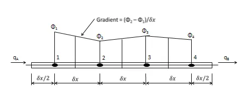
Conservation is ensured in central differencing scheme since overall flux balance is obtained by summing the net flux through each control volume taking into account the boundary fluxes for the control volumes around nodes 1 and 4.

Boundary flux for control volume around node 1 and 4

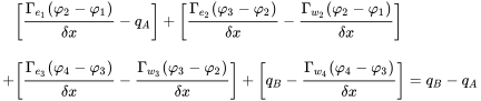
Because,

Boundedness

Central differencing scheme satisfies first condition of boundedness

Since }

from continuity equation, therefore;

Another essential requirement for boundedness is that all coefficients of the discretised equations should have the same sign (usually all positive).

But this is only satisfied when peclect number

because for a unidirectional flow() a is always positive if

Transportiveness

It requires that transportiveness changes according to magnitude of peclet number i.e. when pe is zero is spread in all directions equally and as Pe increases (convection > diffusion) at a point largely depends on upstream value and less on downstream value. But central differencing scheme does not possess transportiveness at higher pe since Φ at a point is average of neighbouring nodes for all Pe.

Accuracy

The taylor series truncation error of the central differencing scheme is second order. Central differencing scheme will be accurate only if Pe < 2. Owing to this limitation, central differencing is not a suitable discretisation practice for general purpose flow calculations.

Applications

• They are currently used on a regular basis in the solution of the Euler Equations and Navier Stokes Equations.
• Results using central differencing approximation have shown noticeable improvements in accuracy in smooth regions.
• Shock wave representation and Boundary layer definition can be improved on coarse meshes.

Advantages

• Simpler to program, requires less computer time per step, and works well with multigrid accleration techniques
• Has a free parameter in conjunction with the fourth-difference dissipation, which is needed to approach a steady state.
• More accurate than the first-order upwind scheme if the Peclet number is less than 2.

Disadvantages

• Somewhat more dissipative

• Leads to oscillations in the solution or divergence if the local Peclet number is larger than 2

Upwind Scheme

The upwind differencing scheme is a method used in numerical methods in computational fluid dynamics for convection diffusion problems. This scheme is specific for peclect number greater than 2 or less than −2

By taking into account the direction of the flow, the upwind differencing scheme overcomes that inability of the central diffrencing scheme. This scheme is developed for strong convective flows with suppressed diffusion effects. Also known as ‘Donor Cell’ Differencing Scheme, the convected value of property at the cell face is adopted from the upstream node.

It can be described by Steady convection-diffusion partial Differential Equation

Peclet number:

It is non dimensional number and it determining comparitive strength of convection and diffusion

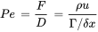
For positive flow direction

Corresponding upwind scheme equation:

-----(3)

Due to strong convection and suppressed diffusion

Rearranging equation (3) gives

]

Identifying coefficients,

For negative flow direction

Corresponding upwind scheme equation:

----(4)

Rearranging equation(4) gives

Identifying coefficients,

We can generalize coefficients as

Conservativeness

The upwind differencing scheme formulation is conservative.

Boundedness

As the coefficients of the discretised equation are always positive hence satisfying the requirements for boundedness and also the coefficient matrix is diagonally dominant therefore no irregularities occur in the solution.

Transportiveness

Transportiveness is built into the formulation as the scheme already accounts for the flow direction.

Accuracy

Based on the backward differencing formula, the accuracy is only first order on the basis of the taylor series truncation error. It gives error when flow is not aligned with grid lines. Distribution of transported properties become marked giving diffusion-like appearance, called as the false diffusion Refinement of grid serves in overcoming the issue of false diffusion. With decrease in the grid size, false diffusion decrease thus increasing the accuracy.

Second order Upwind Scheme(LUD Scheme)

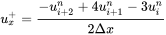
The spatial accuracy of the first-order upwind scheme can be improved by including 3 data points instead of just 2, which offers a more accurate finite difference stencil for the approximation of spatial derivative. For the second-order upwind scheme, becomes the 3-point backward difference in equation and is defined as

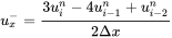
and is the 3-point forward difference, defined as

QUICK Scheme

This scheme is less diffusive compared to the first-order accurate scheme and is called linear upwind differencing (LUD) scheme.

In cfd QUICK, which stands for Quadratic Upstream Interpolation for Convective Kinematics, is a higher-order differencing scheme that considers a three-point upstream weighted quadradtic interpolation for the cell face values. In computational fluid dynamics there are many solution methods for solving the steady state convection diffusion. Some of the used methods are the central differencing scheme, upwind scheme hybrid scheme, power law scheme and QUICK scheme.

Quadratic Interpolation

For the one-dimensional domain shown in the figure the Φ value at a control volume face is approximated using three-point quadratic function passing through the two bracketing or surrounding nodes and one other node on upstream side. In the figure, in order to calculate the value of the property at the face, we should have three nodes i.e. two bracketing or surrounding nodes and one upstream node.

1. Φ_w when u_w > 0 and u_e > 0 a quadratic fit through WW, W and P is used,
2. Φ_e when u_w > 0 and u_e > 0 a quadratic fit through W, P and E is used,
3. Φ_w when u_w < 0 and u_e < 0 values of W, P and E are used,
4. Φ_e when u_w < 0 and u_e < 0 values of P, E and EE are used.

Let the two bracketing nodes be i and i − 1 and upstream node i – 2 then for a uniform grid the value of φ at the cell face between the three nodes is given by:

Interpolation Property

The steady convection and diffusion of a property 'Ƥ' in a given one-dimensional flow field with velocity 'u' and in the absence of sources is given

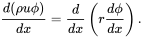
For the continuity of the flow it must also satisfy

Discretizing the above equation to a control volume around a particular node we get

Integrating this continuity equation over the control volume we get

now assuming and

The corresponding cell face values of the above variables are given by

Assuming constant area over the entire control volume we get

Positive Direction

When the flow is in positive direction the values of the velocities will be ,

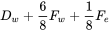
For "w (west face)" bracketing nodes are W and P, the upstream node is WW then,

For "e (east face)" bracketing nodes are P and E, the upstream node is W then

where,

Negative Direction

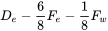
For < 0 and < 0 the flux across the west and east boundaries is given by the expressions :

Quick Scheme for 1D convection Diffusion

a_PΦ_P = a_WΦ_W + a_EΦ_E + a_WWΦ_WW + a_EEΦ_EE

Here, a_P = a_W + a_E + a_WW + a_EE + (F_e - F_w)

other coefficients

aW	aWW	aE	aEE
Dw + 6/8 αw Fw + 1/8Fe αe +3/8 (1 – αw)Fw	−1/8 αwFw	De - 3/8αe Fe -6/8(1–αe)Fe −1/8 (1–αw)Fw	1/8(1 – αe)Fe

where

α_w=1 for F_w > 0 and α_e=1 for F_e > 0

α_w=0 for F_w < 0 and α_e=0 for F_e < 0.

Flux Limiters

• Flux limiters are used in high resolution schemes – numerical schemes used to solve problems in science and engineering, particularly fluid dynamics described by partial diffrential equations (PDE's). They are used in high resolution schemes, such as the MUSUL Scheme to avoid the spurious oscillations (wiggles) that would otherwise occur with high order spatial discretization schemes due to shocks, discontinuities or sharp changes in the solution domain. Use of flux limiters, together with an appropriate high resolution scheme, make the solutions total varition diminishing.
• That flux limiters are also referred to as slope limiters because they both have the same mathematical form, and both have the effect of limiting the solution gradient near shocks or discontinuities. In general, the term flux limiter is used when the limiter acts on system fluxes and slope limiter is used when the limiter acts on system states (like pressure, velocity etc.).
• The main idea behind the construction of flux limiter schemes is to limit the spatial derivatives to realistic values – for scientific and engineering problems this usually means physically realisable and meaningful values. They are used in high resolution schemes for solving problems described by PDEs and only come into operation when sharp wave fronts are present. For smoothly changing waves, the flux limiters do not operate and the spatial derivatives can be represented by higher order approximations without introducing spurious oscillations. Consider the 1D semi discrete scheme below,

where, and represent edge fluxes for the ith cell. If these edge fluxes can be represented by low and high resolution schemes, then a flux limiter can switch between these schemes depending upon the gradients close to the particular cell, as follows,

,

,

where

low resolution flux,

high resolution flux,

flux limiter function,

and represents the ratio of successive gradients on the solution mesh,

.

The limiter function is constrained to be greater than or equal to zero, . Therefore, when the limiter is equal to zero (sharp gradient, opposite slopes or zero gradient), the flux is represented by a low resolution scheme. Similarly, when the limiter is equal to 1 (smooth solution), it is represented by a high resolution scheme. The various limiters have differing switching characteristics and are selected according to the particular problem and solution scheme. No particular limiter has been found to work well for all problems, and a particular choice is usually made on a trial and error basis.