Week 5.1 - Mid term project - Solving the steady and unsteady 2D heat conduction problem
Aim
To write and solve the steady and unsteady two dimensional heat conduction Equation by using MATLAB
Given Data
Solve the 2D heat conduction equation by using the point iterative techniques that were taught in the class. The Boundary conditions for the problem are as follows;
Top Boundary = 600 K
Bottom Boundary = 900 K
Left Boundary = 400 K
Right Boundary = 800 K
Your absolute error criteria is 1e-4
You will implement the following methods for solving implicit equations.
1. Jacobi
2. Gauss-seidel
3. Successive over-relaxation (SOR)
Introduction
Thermal conduction is the transfer of internal energy by microscopic collisions of particles and the movement of electrons within a body. The collision leads to the transfer of the internal energy whether it be Kinetic energy or Potential Energy.
The 2D Heat equation ∂T/∂t -∝(∂^2T/∂x^2 + ∂^2T/∂y^2) = 0
Steady State Condition
A form of conduction that happens when the temperature difference driving the conduction is constant so that the spatial distribution of temperatures in the conducting object does not change any further. So the spatial temperature derivative is constant and the time-temperature derivative is zero.
(∂^2T/∂x^2 + ∂^2T/∂y^2) = 0
Unsteady State Condition
A form of conduction in which the time-dependent temperature derivative is non-zero and affects the overall temperature and the conduction in a system, and temperature changes in time toward a new equilibrium. It can be considered that new sources and sinks are suddenly introduced in a pre-existing system at the boundary.
As the equilibrium is attained the system returns to the original condition and the Heat energy remains conserved.
∂T/∂t -α(∂^2T/∂x^2 + ∂2^T/∂y^2) = 0
STEADY STATE CONDITION
Jacobi Method,
2* TP ((1/△x^2) + (1/△y^2)) =( (TL + TR)/△x^2) + ( ( TT + TB )/△y^2)
k = 2*[(1/△x^2) + (1/△y^2)]
Tn+1P = (1/k) * ( (TL + TR)/△x^2) + ( ( TT + TB )/△y^2)n
Gauss seidel,
Tn+1P = (1/k) * ( (TL + TR)/△x^2) + ( ( TT + TB )/△y^2)n + 1
SOR,
Tn+1P = (1 - w)*TnP w * ( (TL + TR)/△x^2) + ( ( TT + TB )/△y^2)n + 1
clear all
close all
clc

% inputs
L=1;
nx = 20;
ny = 20;

% x and y grid
x = linspace(0,L,nx);
y = linspace(0,L,ny);
[X,Y] = meshgrid(x,y);
dx = L/(nx - 1);
dy = L/(ny - 1);

% Error and Tolerence
error = 9e9;
tolerance = 1e-4;

% Temperature
T_L = 400;
T_T = 600;
T_R = 800;
T_B = 900;

T = ones(nx,ny);

% Assign the Temperature Values
T (2:ny-1,1) = T_L;
T (2:ny-1,nx) = T_R;
T (1,2:nx-1) = T_T;
T (ny,2:nx-1) = T_B;

% Calculate corner temperature values
T(1,1) = (T_T + T_L)/2;
T(nx,ny) = (T_R + T_B)/2;
T(1,ny) = (T_T + T_R)/2;
T(nx,1) = (T_L + T_B)/2;

% Value of Original array
T_initial = T;
T_old = T;

alpha = 0.5;
t = 5;
dt = 1e-2;

k = 2*((1/dx^2) + (1/dy^2));
k1 = alpha *(dt/dx^2);
k2 = alpha *(dt/dy^2);

% jacobi method
jacobi_iteration = 1;
tic
while (error > tolerance)
    for i= 2:nx-1
        for j = 2:ny-1
            term1 = (T_old(i-1,j) + T_old(i+1,j))/(k*(dx^2));
            term2 = (T_old(i,j-1) + T_old(i,j+1))/(k*(dy^2));
            T(i,j) = term1 + term2;
        end
    end
    error = max(max(abs(T_old - T)));
    T_old = T;
    jacobi_iteration = jacobi_iteration + 1;
end
iteration_time = toc;

% plottings
figure(1)
[a,b] = contourf (X, Y, T);
set(gca, 'YDIR','reverse')
colormap(jet)
clabel(a,b)
xlabel( 'X Length')
ylabel('Y Length')
text1 = sprintf('Iteration = %d',jacobi_iteration);
text2 = sprintf('Simulation time = %f s',iteration_time);
text3 = sprintf('Final error = %f',error);
colorbar
title ({'Jacobi Method for Steady State';text1;text2;text3})

% % Gauss Seidel Method

gauss_seidel_iteration = 1;
tic
while (error > tolerance)
    for i= 2:nx-1
        for j = 2:ny-1
            term1 = (T(i-1,j) + T_old(i+1,j))/(k*(dx^2));
            term2 = (T(i,j-1) + T_old(i,j+1))/(k*(dy^2));
            T(i,j) = term1 + term2;
        end
    end
    error = max(max(abs(T_old - T)));
    T_old = T;
    gauss_seidel_iteration = gauss_seidel_iteration + 1;
end
iteration_time = toc;

% plottings
figure(2)
[a,b] = contourf (X, Y, T);
set(gca, 'YDIR','reverse')
colormap(jet)
clabel(a,b)
xlabel( 'X Length')
ylabel('Y Length')
text1 = sprintf('Iteration = %d',gauss_seidel_iteration);
text2 = sprintf('Simulation time = %f s',iteration_time);
text3 = sprintf('Final error = %f',error);
colorbar
title ({'Gauss Seidel Method for Steady State';text1;text2;text3})

% % SOR Method
w=1.5;
SOR_iteration = 1;
tic
while (error > tolerance)
    for i= 2:nx-1
        for j = 2:ny-1
            term1 = (T(i-1,j) + T_old(i+1,j))/(k*(dx^2));
            term2 = (T(i,j-1) + T_old(i,j+1))/(k*(dy^2));
            T(i,j) = (1-w)*T_old(i,j) + (term1 + term2)*w;
        end
    end
    error = max(max(abs(T_old - T)));
    T_old = T;
    SOR_iteration = SOR_iteration + 1;
end
iteration_time = toc;

% plottings
figure(2)
[a,b] = contourf (X, Y, T);
set(gca, 'YDIR','reverse')
colormap(jet)
clabel(a,b)
xlabel( 'X Length')
ylabel('Y Length')
text1 = sprintf('Iteration = %d',SOR_iteration);
text2 = sprintf('Simulation time = %f s',iteration_time);
text3 = sprintf('Final error = %f',error);
colorbar
title ({'SOR Method for Steady State';text1;text2;text3})
Results
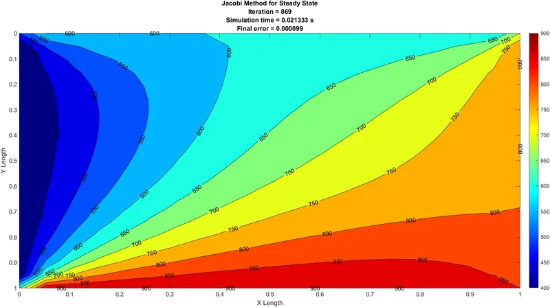
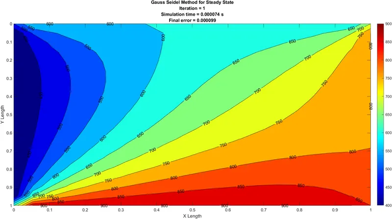
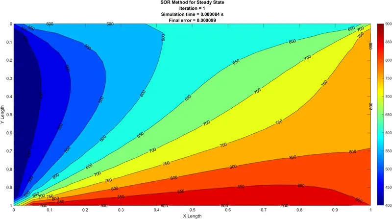
Conclusion
- The Convergence is faster in terms of time and iteration in the case of SOR method than Gauss Seidel and Jacobi Method and the error observes a considerable drop as well.
Transient Implicit Condition
A fluid state in which there is a change in fluid properties concerning time is an unsteady state Transient State.
∂T/∂t -(∂^2T/∂x^2 + ∂^2T/∂y^2) = 0
Implicit
Jacobi
TPn + 1 = [TPn+ K1 (TLn + TRn) +K2 ( TTn+ TBn ) ] / (1 + 2*K1 + 2*K2)
Gauss seidel
TPn + 1 = [TPn+ K1 (TLn + 1 + TRn + 1) +K2 ( TTn + 1+ TBn + 1 ) ] / (1 + 2*K1 + 2*K2)
SOR,
TPn + 1 =[[TPn+ K1 (TLn + 1 + TRn + 1) +K2 ( TTn + 1+ TBn + 1 ) ] / (1 + 2*K1 + 2*K2)]*w + (TPn)(1-w)
clear all
close all
clc

% inputs
L=1;
nx = 20;
ny = 20;

% x and y grid
x = linspace(0,L,nx);
y = linspace(0,L,ny);
[X,Y] = meshgrid(x,y);
dx = L/(nx - 1);
dy = L/(ny - 1);

% Error and Tolerence
error = 9e9;
tolerance = 1e-4;

% Temperature
T_L = 400;
T_T = 600;
T_R = 800;
T_B = 900;

T = ones(nx,ny);

% Assign the Temperature Values
T (2:ny-1,1) = T_L;
T (2:ny-1,nx) = T_R;
T (1,2:nx-1) = T_T;
T (ny,2:nx-1) = T_B;

% Calculate corner temperature values
T(1,1) = (T_T + T_L)/2;
T(nx,ny) = (T_R + T_B)/2;
T(1,ny) = (T_T + T_R)/2;
T(nx,1) = (T_L + T_B)/2;

% Value of Original array
T_initial = T;
T_old = T;

alpha = 0.5;
t = 5;
dt = 1e-2;

k = 2*((1/dx^2) + (1/dy^2));
k1 = alpha *(dt/dx^2);
k2 = alpha *(dt/dy^2);

% %  Jacobi Method for Transient - Implicit

nt = t/dt;
implicit_jacobi_iteration = 1;
T_pre = T;
tic
for m = 1:nt
    error = 9e9;
    while (error > tolerance)
        for i = 2:nx-1
            for j = 2:ny-1
                term1 = (T_old(i-1,j) + T_old(i+1,j));
                term2 = (T_old(i,j-1) + T_old(i,j+1));
                T(i,j) = (T_pre(i,j) + (k1*term1) + (k2*term2))/(1+ 2*k1 + 2*k2);
            end
        end
        error = max(max(abs(T_old - T)));
        T_old = T;
        implicit_jacobi_iteration = implicit_jacobi_iteration + 1;
    end
    T_pre = T;
end
iteration_time = toc;

% plottings

figure(4)
[a,b] = contourf (X, Y, T);
set(gca, 'YDIR','reverse')
colormap(jet)
clabel(a,b)
xlabel( 'X Length')
ylabel('Y Length')
text1 = sprintf('Iteration = %d',implicit_jacobi_iteration);
text2 = sprintf('Simulation time = %f s',iteration_time);
text3 = sprintf('Final error = %f',error);
colorbar
title ({'Jacobi Method for Transient State Implicit';text1;text2;text3})

% % Gauss seidel Method for Transient Implicit
nt = t/dt;
implicit_gauss_seidel_iteration = 1;
T_pre = T;
tic
for m = 1:nt
    error = 9e9;
    while (error > tolerance)
        for i = 2:nx-1
            for j = 2:ny-1
                term1 = (T(i-1,j) + T_old(i+1,j));
                term2 = (T(i,j-1) + T_old(i,j+1));
                T(i,j) = (T_pre(i,j) + (k1*term1) + (k2*term2))/(1+ 2*k1 + 2*k2);
            end
        end
        error = max(max(abs(T_old - T)));
        T_old = T;
        implicit_gauss_seidel_iteration = implicit_gauss_seidel_iteration + 1;
    end
    T_pre = T;
end
iteration_time = toc;

% plottings

figure(5)
[a,b] = contourf (X, Y, T);
set(gca, 'YDIR','reverse')
colormap(jet)
clabel(a,b)
xlabel( 'X Length')
ylabel('Y Length')
text1 = sprintf('Iteration = %d',implicit_gauss_seidel_iteration);
text2 = sprintf('Simulation time = %f s',iteration_time);
text3 = sprintf('Final error = %f',error);
colorbar
title ({'Gauss Seidel Method for Transient State Implicit';text1;text2;text3})


% % SOR Method for Transient Implicit condition

nt = t/dt;
implicit_SOR_iteration = 1;
T_pre = T;
w=1.5;
tic
for m = 1:nt
    error = 9e9;
    while (error > tolerance)
        for i = 2:nx-1
            for j = 2:ny-1
                term1 = (T(i-1,j) + T_old(i+1,j));
                term2 = (T(i,j-1) + T_old(i,j+1));
                T(i,j) = (1-w)*T_old(i,j) + (w*(T_pre(i,j) + (k1*term1) + (k2*term2)))/(1+ 2*k1 + 2*k2);
            end
        end
        error = max(max(abs(T_old - T)));
        T_old = T;
        implicit_SOR_iteration = implicit_SOR_iteration + 1;
    end
    T_pre = T;
end
iteration_time = toc;

% plottings

figure(6)
[a,b] = contourf (X, Y, T);
set(gca, 'YDIR','reverse')
colormap(jet)
clabel(a,b)
xlabel( 'X Length')
ylabel('Y Length')
text1 = sprintf('Iteration = %d',implicit_SOR_iteration);
text2 = sprintf('Simulation time = %f s',iteration_time);
text3 = sprintf('Final error = %f',error);
colorbar
title ({'SOR Method for Transient State Implicit';text1;text2;text3})
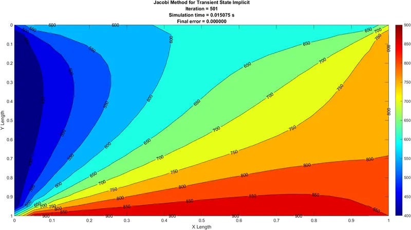
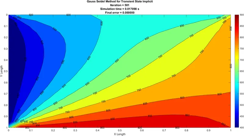
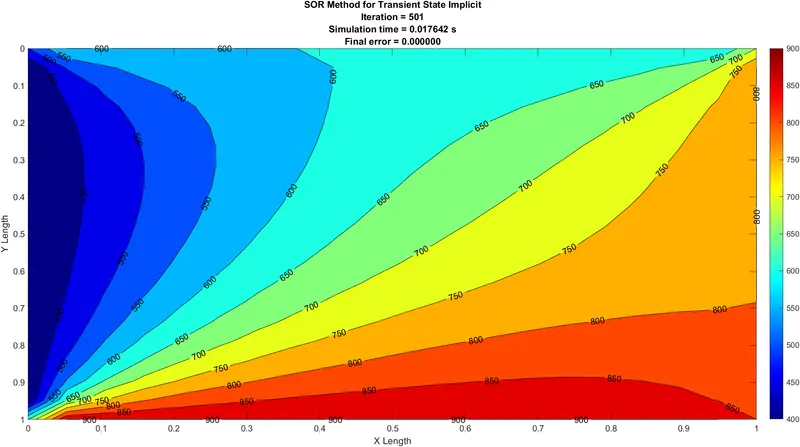
Conclusion
- The number of iterations in the implicit solver in unsteady state is noticeably more than that of explicit solver.
- The SOR method is faster in terms of iterations computed and in terms of simulation time and the error is negligible.
For Transient Explicit
Explicit
Jacobi,
TPn + 1 = [ (1 - 2*K1 - 2*K2)TPn+ K1 (TLn + TRn) +K2 ( TTn+ TBn ) ]
Gauss,
TPn + 1 = [ (1 - 2*K1 - 2*K2)TPn+ K1 (TLn + 1 + TRn + 1) +K2 ( TTn + 1+ TBn + 1 ) ]
SOR,
TPn + 1 =[TPn (1 - 2*K1 - 2*K2)+ K1 (TLn + 1 + TRn + 1) +K2 ( TTn + 1+ TBn + 1 ) ]*w + (TPn)(1-w)
clear all
close all
clc

% inputs
L=1;
nx = 20;
ny = 20;

% x and y grid
x = linspace(0,L,nx);
y = linspace(0,L,ny);
[X,Y] = meshgrid(x,y);
dx = L/(nx - 1);
dy = L/(ny - 1);

% Error and Tolerence
error = 9e9;
tolerance = 1e-4;

% Temperature
T_L = 400;
T_T = 600;
T_R = 800;
T_B = 900;

T = ones(nx,ny);

% Assign the Temperature Values
T (2:ny-1,1) = T_L;
T (2:ny-1,nx) = T_R;
T (1,2:nx-1) = T_T;
T (ny,2:nx-1) = T_B;

% Calculate corner temperature values
T(1,1) = (T_T + T_L)/2;
T(nx,ny) = (T_R + T_B)/2;
T(1,ny) = (T_T + T_R)/2;
T(nx,1) = (T_L + T_B)/2;

% Value of Original array
T_initial = T;
T_old = T;

alpha = 0.5;
t = 5;
dt = 1e-2;

k = 2*((1/dx^2) + (1/dy^2));
k1 = alpha *(dt/dx^2);
k2 = alpha *(dt/dy^2);

% % Jacobi Method for Transient Explicit
[X,Y] = meshgrid(x,y);
nt = t/dt;
explicit_jacobi_iteration = 1;
T_pre = T;
tic
for m = 1:nt
    error = 9e9;
    while (error > tolerance)
        for i = 2:nx-1
            for j = 2:ny-1
                term1 = (T_old(i-1,j) + T_old(i+1,j));
                term2 = (T_old(i,j-1) + T_old(i,j+1));
                T(i,j) = (T_pre(i,j) + (k1*term1) + (k2*term2))/(1+ 2*k1 + 2*k2);
            end
        end
        error = max(max(abs(T_old - T)));
        T_old = T;
        explicit_jacobi_iteration = explicit_jacobi_iteration + 1;
    end
    T_pre = T;
end
iteration_time = toc;

% plottings

figure(7)
[a,b] = contourf (X, Y, T);
set(gca, 'YDIR','reverse')
colormap(jet)
clabel(a,b)
xlabel( 'X Length')
ylabel('Y Length')
text1 = sprintf('Iteration = %d',explicit_jacobi_iteration);
text2 = sprintf('Simulation time = %f s',iteration_time);
text3 = sprintf('Final error = %f',error);
colorbar
title ({'Jacobi Method for Transient State Explicit';text1;text2;text3})

% % Gauss seidel Method for Transient Explicit
nt = t/dt;
explicit_gauss_seidel_iteration = 1;
T_pre = T;
tic
for m = 1:nt
    error = 9e9;
    while (error > tolerance)
        for i = 2:nx-1
            for j = 2:ny-1
                term1 = (T(i-1,j) + T_old(i+1,j));
                term2 = (T(i,j-1) + T_old(i,j+1));
                T(i,j) = (T_pre(i,j) + (k1*term1) + (k2*term2))/(1+ 2*k1 + 2*k2);
            end
        end
        error = max(max(abs(T_old - T)));
        T_old = T;
        explicit_gauss_seidel_iteration = explicit_gauss_seidel_iteration + 1;
    end
    T_pre = T;
end
iteration_time = toc;

% plottings

figure(8)
[a,b] = contourf (X, Y, T);
set(gca, 'YDIR','reverse')
colormap(jet)
clabel(a,b)
xlabel( 'X Length')
ylabel('Y Length')
text1 = sprintf('Iteration = %d',explicit_gauss_seidel_iteration);
text2 = sprintf('Simulation time = %f s',iteration_time);
text3 = sprintf('Final error = %f',error);
colorbar
title ({'Gauss Seidel Method for Transient State Explicit';text1;text2;text3})

% % SOR Method for Transient Explicit condition

nt = t/dt;
explicit_SOR_iteration = 1;
T_pre = T;
w=1.5;
tic
for m = 1:nt
    error = 9e9;
    while (error > tolerance)
        for i = 2:nx-1
            for j = 2:ny-1
               term1 = (T(i-1,j) + T_old(i+1,j));
                term2 = (T(i,j-1) + T_old(i,j+1));
                T(i,j) = (1-w)*T_old(i,j) + (w*(T_pre(i,j) + (k1*term1) + (k2*term2)))/(1+ 2*k1 + 2*k2);
            end
        end
        error = max(max(abs(T_old - T)));
        T_old = T;
        explicit_SOR_iteration = explicit_SOR_iteration + 1;
    end
    T_pre = T;
end
iteration_time = toc;

% plottings

figure(6)
[a,b] = contourf (X, Y, T);
set(gca, 'YDIR','reverse')
colormap(jet)
clabel(a,b)
xlabel( 'X Length')
ylabel('Y Length')
text1 = sprintf('Iteration = %d',explicit_SOR_iteration);
text2 = sprintf('Simulation time = %f s',iteration_time);
text3 = sprintf('Final error = %f',error);
colorbar
title ({'SOR Method for Transient State Explicit';text1;text2;text3})
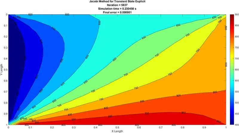
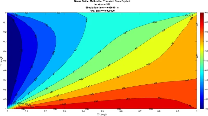
Conclusion
- In the explicit method the stability is mostly dependent upon the CFL number which should be less than 0.5.
- The time step plays a very important role in the stability of the solution as the time step increases the CFL number increases.
- In an implicit method the solution is stable and hence there is no effect of the CFL number on the stability of the solution, which allows the use of large timesteps.