Week 3.5 - Deriving 4th order approximation of a 2nd order derivative using Taylor Table method

Aim

Derive the following 4th order approximations of the second-order derivative.

1. Central difference

2. Skewed right-sided difference

3. Skewed left-sided difference

and compare the numerical approximations by using matlab

Introduction

Taylor series

f(x+dx) = f(x) +h/1!. f'(x)+h^2/2!.f"(x)+h^3/3!.f"'(x)+h^4/4!.f""(x)+.........

the above series used to approximate the derivatives from the neighbouring points, then the approximation have some errors.

here we dealing with three types of schemes they are skewed right dide scheme,skewed left side scheme and central diffrence scheme.

here we used taylor table method

for central scheme

no of nodes P+Q-1 =2+4-1 =5

for skewed schemes

no of nodes = P+Q = 2+4 =6

1. Central difrence Scheme

f(x)	a	0	0	0	0
f(x+dx)	b	b	b/2	b/6	b/24
f(x+2dx)	c	2*c	2*c	4c/3	2c/3
f(x-dx)	d	-d	d/2	-d/6	d/24
f(x-2dx)	e	-2e	2e	-4e/3	2*e/3

>> AC=[1 1 1 1 1; -2 -1 0 1 2; 4/2 1/2 0 1/2 4/2; -8/6 -1/6 0 1/6 8/6; 16/24 1/24 0 1/24 16/24]

AC =

    1.0000    1.0000    1.0000    1.0000    1.0000
   -2.0000   -1.0000         0    1.0000    2.0000
    2.0000    0.5000         0    0.5000    2.0000
   -1.3333   -0.1667         0    0.1667    1.3333
    0.6667    0.0417         0    0.0417    0.6667

>> BC=[0;0;1;0;0]

BC =

     0
     0
     1
     0
     0

>> xc=inv(AC)*BC

xc =

   -0.0833
    1.3333
   -2.5000
    1.3333
   -0.0833

Skewed Right side diffrence

f"(x)=a.f(x)+b.f(x+dx)+c.f(x+2dx)...../dx^2

f(x)	a	0	0	0	0	0
f(x+dx)	b	b	b/2	b/6	b/24	b/120
f(x+2dx)	c	2c	2c	4c/3	2c/3	4c/15
f(x+3dx)	d	3d	9d/2	9d/2	27d/8	81d/40
f(x+4dx)	e	4e	8e	32e/3	32e/3	128e/15
f(x+5dx)	g	5g	25g/2	125g/6	625g/24	625g/24

>> AR=[1 1 1 1 1 1; 0 1 2 3 4 5; 0 1/2 4/2 9/2 16/2 25/2; 0 1/6 8/6 27/6 64/6 125/6; 0 1/24 16/24 81/24 256/24 625/24; 0 1/120 32/120 243/120 1024/120 3125/120]

AR =

    1.0000    1.0000    1.0000    1.0000    1.0000    1.0000
         0    1.0000    2.0000    3.0000    4.0000    5.0000
         0    0.5000    2.0000    4.5000    8.0000   12.5000
         0    0.1667    1.3333    4.5000   10.6667   20.8333
         0    0.0417    0.6667    3.3750   10.6667   26.0417
         0    0.0083    0.2667    2.0250    8.5333   26.0417

>> BR=[0;0;1;0;0;0]

BR =

     0
     0
     1
     0
     0
     0

>> xr=inv(AR)*BR

xr =

    3.7500
  -12.8333
   17.8333
  -13.0000
    5.0833
   -0.8333

Skewed Left side scheme

f"(x)=a.f(x)+b.f(x-dx)+c.f(x-2dx)...../dx^2

f(x)	a	0	0	0	0	0
f(x-dx)	b	b	b/2	b/6	b/24	b/120
f(x-2dx)	c	2c	2c	4c/3	2c/3	4c/15
f(x-3dx)	d	3d	9d/2	9d/2	27d/8	81d/40
f(x-4dx)	e	4e	8e	32e/3	32e/3	128e/15
f(x-5dx)	g	5g	25g/2	125g/6	625g/24	625g/24

 AL=[1 1 1 1 1 1; 0 -1 -2 -3 -4 -5; 0 1/2 4/2 9/2 16/2 25/2; 0 -1/6 -8/6 -27/6 -64/6 -125/6; 0 1/24 16/24 81/24 256/24 625/24; 0 -1/120 -32/120 -243/120 -1024/120 -3125/120]

AL =

    1.0000    1.0000    1.0000    1.0000    1.0000    1.0000
         0   -1.0000   -2.0000   -3.0000   -4.0000   -5.0000
         0    0.5000    2.0000    4.5000    8.0000   12.5000
         0   -0.1667   -1.3333   -4.5000  -10.6667  -20.8333
         0    0.0417    0.6667    3.3750   10.6667   26.0417
         0   -0.0083   -0.2667   -2.0250   -8.5333  -26.0417

>> BL=[0;0;1;0;0;0]

BL =

     0
     0
     1
     0
     0
     0

>> xl=inv(AL)*BL

xl =

    3.7500
  -12.8333
   17.8333
  -13.0000
    5.0833
   -0.8333

clear all
close all
clc

% inputs
x=pi/3;
dx=linspace(pi/4000,pi/40,20);

% analytical derivative
% f(x) = exp(x)*cos(x)
% f'(x) = (exp(x)*cos(x) - exp(x)*sin(x)) = exp(x)*(cos(x) - sin(x))
% f"(x) = -2 exp(x)*sin(x)
analytical_derivative = -2*exp(x)*sin(x);

% Approximations
% Central Scheme
AC=[1 1 1 1 1; -2 -1 0 1 2; 4/2 1/2 0 1/2 4/2; -8/6 -1/6 0 1/6 8/6; 16/24 1/24 0 1/24 16/24];
BC=[0;0;1;0;0];
xc=inv(AC)*BC;


% Skewed right side diffrence
AR=[1 1 1 1 1 1; 0 1 2 3 4 5; 0 1/2 4/2 9/2 16/2 25/2; 0 1/6 8/6 27/6 64/6 125/6; 0 1/24 16/24 81/24 256/24 625/24; 0 1/120 32/120 243/120 1024/120 3125/120];
BR=[0;0;1;0;0;0];
xr=inv(AR)*BR;

% Skewed left side diffrence
AL=[1 1 1 1 1 1; 0 -1 -2 -3 -4 -5; 0 1/2 4/2 9/2 16/2 25/2; 0 -1/6 -8/6 -27/6 -64/6 -125/6; 0 1/24 16/24 81/24 256/24 625/24; 0 -1/120 -32/120 -243/120 -1024/120 -3125/120];
BL=[0;0;1;0;0;0];
xl=inv(AL)*BL;

for i=1:length(dx)

% Numerical Derivative
central_diffrence(i) = (ac.*exp(x-2.*dx).*cos(x-2.*dx)+bc.*exp(x-dx).*cos(x-dx)+cc.*exp(x).*cos(x)+dc.*exp(x+dx).*cos(x+dx)+ec.*exp(x+2*dx).*cos(x+2.*dx))/((dx).^2);
skewed_right_side_diffrence(i) = (ar.*exp(x).*cos(x)+br.*exp(x+dx).*cos(x+dx)+cr.*exp(x+2.*dx).*cos(x+2.*dx)+dr.*exp(x+3.*dx).*cos(x+3.*dx)+er.*exp(x+4.*dx).*cos(x+4.*dx)+gr.*exp(x+5.*dx).*cos(x+5.*dx))/((dx).^2);
skewed_left_side_diffrence(i) = (al.*exp(x).*cos(x)+bl.*exp(x-dx).*cos(x-dx)+cl.*exp(x-2.*dx).*cos(x-2.*dx)+dl.*exp(x-3.*dx).*cos(x-3.*dx)+el.*exp(x-4.*dx).*cos(x-4.*dx)+gl.*exp(x-5.*dx).*cos(x-5.*dx))/((dx).^2);

% Error
error_central_diffrence(i) = abs(analytical_derivative - central_diffrence);
error_skewed_right_side_diffrence(i) = abs(analytical_derivative - skewed_right_side_diffrence);
error_skewed_left_side_diffrence(i) = abs(analytical_derivative - skewed_left_side__diffrence);
error=[error_central_diffrence(i);skewed_right_side_diffrence(i);skewed_left_side__diffrence(i)];
% Graph plot
figure(1)
loglog(dx,central_diffrence,'r')
hold on
loglog(dx,skewed_right_side_diffrence,'g')
hold on
loglog(dx,skewed_left_side_diffrence,'b')
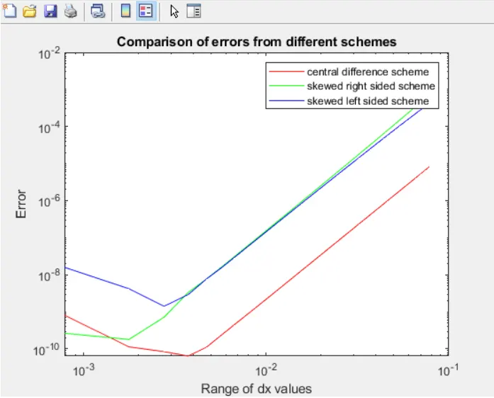
xlabel('Range of dx values')
ylabel('Error')
title('Comparison of errors from diffrent schemes')
legend('central diffrence scheme','skewed right sided scheme','skewed left sided scheme')

Explanation

• First we get the values of a,b,c,d,e,g from the matrix inverse method
• use x and dx values to find the Analytical function and scheme values
• And we need to predict the Analytical function for second order derivative
• by using taylor table method we get the numerical derivative values
• and need to find Error values of schemes
• plot the Graph by using loglog command
• gave label, title and legends to the plot

Result

Conclusion

From the above plot is represnts comparison of error from diffrent schemes, we have calculated the values of diffrent schems As per the plot central scheme error is very low, then the skewed left side and right side diffrence scheme errors is high. and skewed scheme gives same results in the terms.

• Central diffrencing schemes having low order accuracy then it kept as low and it providing proper computational plots and it have symmetric stencil.
• Skewed scheme is useful to predict the boundary condition and it reqiured one direction, then the central schemes need both direction to get the values.