Week 7 - Simulation of a 1D Super-sonic nozzle flow simulation using Macormack Method

Aim

In this challenge i am going to simulate the isentropic flow through a quasi 1D subsonic-supersonic nozzle. Derive both the conservation and non-conservation forms of the governing equations and sovle them using the MacCormack's technique in Matlab

Expected Outputs

1. Steady-state distribution of primitive variables inside the nozzle
2. Time-wise variation of the primitive variables
3. Variation of Mass flow rate distribution inside the nozzle at different time steps during the time-marching process
4. Comparison of Normalized mass flow rate distributions of both forms

Macormack Method

In computational fluid dynamics, the macormack method is a widely used discretization scheme for the numerical solution of hyperbolic partial diffrential equations. This second-order finite diffrence method was introduced by Robert W. MacCormack in 1969.The MacCormack method is elegant and easy to understand and program.

The MacCormack method is a variation of the two step lax wendroff scheme but is much simpler in application. To illustrate the algorithm, consider the following first order hyperbolic equation

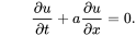
The MacCormack method is well suited for non linear (Inviscid burger's equation and euler's equation etc.) The order of differencing can be reversed for the time step (i.e., forward/backward followed by backward/forward). For nonlinear equations, this procedure provides the best results. For linear equations, the MacCormack scheme is equivalent to the lax wendroff scheme

Unlike first-order upwind scheme, the MacCormack does not introduce diffusive errors in the solution. However, it is known to introduce dispersive errors (gibbs phenomeon) in the region where the gradient is high.

Nozzle

A nozzle is a device designed to control the direction or characteristics of a fluid flow (specially to increase velocity) as it exits (or enters) an enclosed chamber or pipe

A nozzle is often a pipe or tube of varying cross sectional area, and it can be used to direct or modify the flow of a fluid (liquid or Gas). Nozzles are frequently used to control the rate of flow, speed, direction, mass, shape, and/or the pressure of the stream that emerges from them. In a nozzle, the velocity of fluid increases at the expense of its pressure energy.

Assumptions

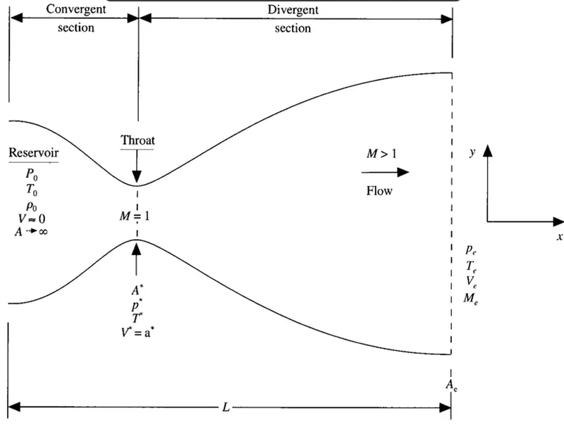
• Here we consider steady, isentrophic flow at Convergent - Divergent Nozzle.
• The flow at the Inlet to the nozzle from the reservoir where the temperature, pressure, Density is denoted as stagnation values.
• The the cross sectional area of reservoir is large
• and the flow exits supersonic flow in nozzle exit .
• the flow is subsonic in convergent section and supersonic in divergent section
• In the sonic speed the local velocity is equal to the local speed of sound

here we assume in the given section the cross sectional area and flow in the uniform section, then the area of nozzle change as a function of distance along with the nozzle

Conservative

clear all
close all
clc

% % Inputs
% Grid Points
n=31;
n1 = 61;
x = linspace(0,3,n);
dx = x(2) - x(1);
x1 = linspace(0,3,n1);

nt = 1400;

% Area
A = 1+2.2*(x-1.5).^2;
A1 = 1+2.2*(x1-1.5).^2;

%% Conservation
gamma = 1.4

% Initial Conditions
for k=1:n
    if x(k)>=0 && x(k)<=0.5
    rho(k) = 1;
    T(k) = 1;
    elseif x(k)>0.5 && x(k)<=1.5
        rho(k) = 1-0.366* (x(k) - 0.5);
        T(k) = 1-0.167* (x(k) - 0.5);
    elseif x(k)>1.5 && x(k)<=3.5
        rho(k) = 0.634-0.3879* (x(k) - 1.5);
        T(k) = 0.833-0.3507* (x(k) - 0.5);
    end
    V = 0.59./(rho.*A);
    U1 = rho.*A;
    U2 = rho.*A.*V;
    U3 = rho.*((T/(gamma-1))+(gamma/2).*V.^2).*A;

% Time Step Calculation
C = 0.5
for i=2:n-1
    timestep (i-1) = C*dx/(T(i)^(1/2)+V(i))
end

dt = min(timestep)

% Time Loop
for t=1:nt

% Store the Initial Values
U1_initial = U1
U2_initial = U2
U3_initial = U3

F1_p = U2
F2_p = (U2.^2./U1)+((gamma-1)/gamma)*(U3-(gamma/2)*(U2.^2./U1))
F3_p = (gamma*U2.*U3./U1)-((gamma*(gamma-1)/2)*U2.^3./U1.^2)

% Maccormack Method for time t
% Predictor time derivative Calculation
dU1dt_p(i) = -(F1_p(i+1)-F1_p(i))/dx
J2_p(i) = (1/gamma)*rho(i).*T(i).*(A(i+1)-A(i))/dx
dU2dt_p(i) = -((F2_p(i+1)-F2_p(i))/dx)+J2_p(i)
dU3dt_p(i) = -(F3_p(i+1)-F3_p(i))/dx

% Update the values
U1(i) = U1(i)+dU1dt_p(i)*dt
U2(i) = U2(i)+dU2dt_p(i)*dt
U3(i) = U3(i)+dU3dt_p(i)*dt
end

% Predictor Loop
rho = U1./A
T = (gamma-1)*(U3./U1-(gamma/2)*(U2./U1).^2)
F1_c = U2
F2_c = (U2.^2./U1)+((gamma-1)/gamma)*(U3-(gamma/2)*(U2.^2./U1))
F3_c = (gamma*U2.*U3./U1)-((gamma*(gamma-1)/2)*U2.^3./U1.^2)

for i=2:n-1
    dU1dt_c(i) = -(F1_c(i)-F1_p(i-1))/dx
    J2_c(i) = (1/gamma)*rho(i).*T(i).*(A(i)-A(i-1))/dx
    dU2dt_c(i) = -((F2_c(i)-F2_c(i-1))/dx)+J2_c(i)
    dU3dt_c(i) = -(F3_c(i)-F3_c(i-1))/dx
% Average time derivative calculation
dU1dt_avg(i) = 0.5*(dU1dt_c(i)+dU1dt_p(i))
dU2dt_avg(i) = 0.5*(dU2dt_c(i)+dU2dt_p(i))
dU3dt_avg(i) = 0.5*(dU3dt_c(i)+dU3dt_p(i))

U1(i) = U1_initial(i)+dU1dt_avg(i)*dt
U2(i) = U2_initial(i)+dU2dt_avg(i)*dt
U3(i) = U3_initial(i)+dU3dt_avg(i)*dt
end
% Boundary Conditions at Inlet
U1(1) = rho(1)*A(1)
U2(1) = 2*U2(2) - U2(3)
U3(1) = U2(1)/(rho(1)*A(1))
% Boundary Conditions at Outlet
U1(n) = 2*U1(n-1)-U1(n-2)
U2(n) = 2*U2(n-1)-U2(n-2)
U3(n) = 2*U3(n-1)-U3(n-2)

rho =U1./A
V = U2./U1
T = (gamma-1)*((U3./U1)-(gamma/2)*V.^2)
M = V./T.^(1/2)
P = rho.*T

% Time step at i=15
rho_15(t) = rho(15)
T_15(t) = T(15)
V_15(t) = V(15)
end

% Plottings
figure(1)
subplot(5,1,1)
plot(x,V)
xlabel('Nozzle length')
ylabel('Velocity')
title('Steady state primitive variable profiles')
subplot(5,1,2)
plot(x,rho)
xlabel('Nozzle length')
ylabel('Velocity')
subplot(5,1,3)
plot(x,T)
xlabel('Nozzle length')
ylabel('Velocity')
subplot(5,1,4)
plot(x,P)
xlabel('Nozzle length')
ylabel('Velocity')
subplot(5,1,5)
plot(x,M)
xlabel('Nozzle length')
ylabel('Velocity')

figure(2)
subplot(5,1,1)
plot(x,V_c)
xlabel('Time step')
ylabel('Velocity')
title('Transient variation of primitive variable at throat')
subplot(5,1,2)
plot(x,rho_c)
xlabel('Time step')
ylabel('Velocity')
subplot(5,1,3)
plot(x,T_c)
xlabel('Time step')
ylabel('Velocity')
subplot(5,1,4)
plot(x,P_c)
xlabel('Time step')
ylabel('Velocity')
subplot(5,1,5)
plot(x,M_c)
xlabel('Time step')
ylabel('Velocity')

figure(3)
hold on
if k==1
    plot(x,M_c)
end
if k==50
    plot(x,M_c)
end
if k==250
    plot(x,M_c)
end
if k==500
    plot(x,M_c)
end
if k==750
    plot(x,M_c)
end
xlabel('Nozzle length')
ylabel('Mass flow rate')
title('Variation of mass flow rate at diffrent time steps')
legends('1dt','50dt','250dt','500dt','750dt','1200dt')

Non Conservative

clear all
close all
clc

% % Inputs
% Grid Points
n=31;
n1 = 61;
x = linspace(0,3,n);
dx = x(2) - x(1);
x1 = linspace(0,3,n1);

nt = 1400;

% Area
A = 1+2.2*(x-1.5).^2;
A1 = 1+2.2*(x1-1.5).^2;

%% Non Conservation

% Initial Condition
rho = 1-0.3146*x;
T = 1-0.2314*x;
V = (0.1+1.09*x).*T.^(1/2);

% Boundary Conditions
V(n) = 2*V(n-1)-V(n-2);
rho(n) = 2*T(n-1) - T(n-2);

% Time Step calculation
C = 0.5;
for i=1:n
    timestep(i) = C*dx/(T(i)^(1/2)+V(i));

end
dt =min(timestep);
gamma = 1.4;

% time loop
for t=1:nt
   % Store the Initial Values
   rho_initial = rho;
   V_initial = V;
   T_initial = T;
   % Maccormack Method for time t
   for i=2:n-1
       drhodx = (rho(i+1)-rho(i))/dx;
       dVdx = (V(i+1)-V(i))/dx;
       dlnAdx = (log(A(i+1))-log(A(i)))/dx;
       dTdx = (T(i+1)-T(i))/dx;

       % Predictor time calculation
       drhodt_p = -rho(i)*dVdx-rho(i)*V(i)*dlnAdx-V(i)*drhodx;
       dVdt_p = -V(i)*dVdx-(1/gamma)*(dTdx+(T(i)/rho(i))*drhodx);
       dTdx_p = -V(i)*dTdx-(gamma-1)*T(i)*(dVdx+V(i)*dlnAdx);

       % Solution Updating
       rho(i) = rho(i)+drhodt_p*dt;
       V(i) = V(i)+dVdt_p*dt;
       T(i) = T(i)+dTdx_p*dt;
       %  BDS
       drhodx_c = (rho(i)-rho(i-1))/dx;
       dVdx_c = (V(i)-V(i-1))/dx;
       dlnAdx_c = (log(A(i))-log(A(i-1)))/dx;
       dTdx_c = (T(i)-T(i-1))/dx;

       % Calculate corrector time derivatives
       drhodt_c = -rho(i)*dVdx_c-rho(i)*V(i)*dlnAdx_c-V(i)*drhodx_c;
       dVdt_c = -V(i)*dVdx_c-(1/gamma)*(dTdx_c+(T(i)/rho(i))*drhodx_c);
       dTdt_c = -V(i)*dTdx_c-(gamma-1)*T(i)*(dVdx_c+V(i)*dlnAdx_c);
       %  Average time derivatives
       drhodt_avg = 0.5*(drhodt_p+drhodt_c);
       dVdt_avg = 0.5*(dVdt_p+dVdt_c);
       dTdt_avg = 0.5*(dTdx_p+dTdx_c);
       % Calculating final Solution
       rho(i) = rho_initial(i)+drhodt_avg*dt;
       V(i) = V_initial(i)+dVdt_avg*dt;
       T(i) = T_initial(i)+dTdt_avg*dt;
   end
   M = V./T.^(1/2);
   P= rho.*T;
end

% Plottings

figure(1)
subplot(5,1,1)
plot(x,V)
xlabel('Nozzle length')
ylabel('Velocity')
title('Steady state primitive variable profiles')
subplot(5,1,2)
plot(x,rho)
xlabel('Nozzle length')
ylabel('Velocity')
subplot(5,1,3)
plot(x,T)
xlabel('Nozzle length')
ylabel('Velocity')
subplot(5,1,4)
plot(x,P)
xlabel('Nozzle length')
ylabel('Velocity')
subplot(5,1,5)
plot(x,M)
xlabel('Nozzle length')
ylabel('Velocity')

figure(2)
subplot(5,1,1)
plot(x,V_nc)
xlabel('Time step')
ylabel('Velocity')
title('Transient variation of primitive variable at throat')
subplot(5,1,2)
plot(x,rho_nc)
xlabel('Time step')
ylabel('Velocity')
subplot(5,1,3)
plot(x,T_nc)
xlabel('Time step')
ylabel('Velocity')
subplot(5,1,4)
plot(x,P_nc)
xlabel('Time step')
ylabel('Velocity')
subplot(5,1,5)
plot(x,M_nc)
xlabel('Time step')
ylabel('Velocity')

figure(3)
hold on
if k==1
    plot(x,M_nc)
end
if k==50
    plot(x,M_nc)
end
if k==250
    plot(x,M_nc)
end
if k==500
    plot(x,M_nc)
end
if k==750
    plot(x,M_nc)
end
xlabel('Nozzle length')
ylabel('Mass flow rate')
title('Variation of mass flow rate at diffrent time steps')
legends('1dt','50dt','250dt','500dt','750dt','1200dt')

Results

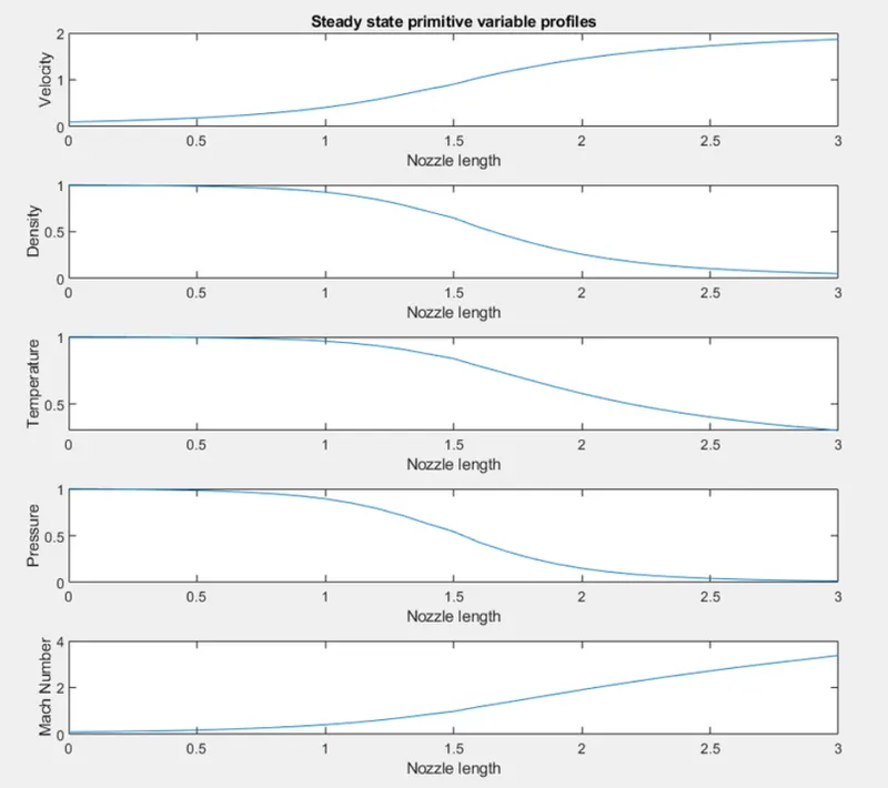
1. Stesdy state distribution of primitive variables inside nozzle

Conservative

Non - Conservative

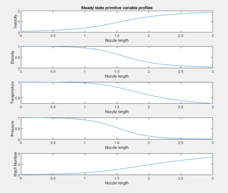
from the above plot, we can observe velocity, density, temperature, pressure and mach number, here the velocity and mach number will be increase from inlet to nozzle. then the pressure, temperature and density will be drop fom inlet to nozzle. According to the bernolli's equation the horizontal flow takes place the velocity will be increase and pressure is decreases and the Analytical solutions referred in Anderson cfd book.

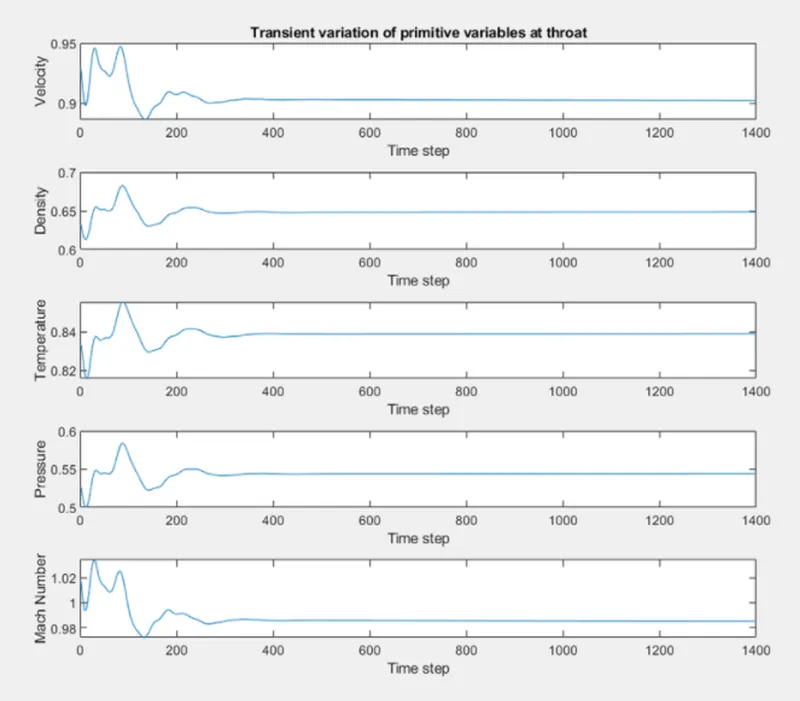
2. Time wise variation at throat

Conservative

Non conservative

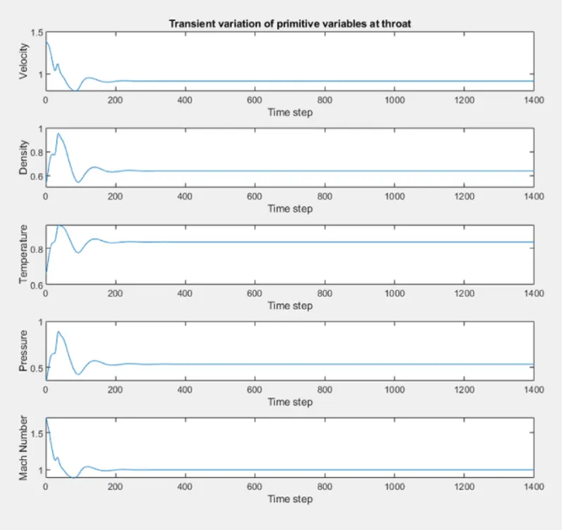
From the above plot we can observe time vise variation in both forms, conservative and non conservative is in steady state condition , the the oscillation are reduced, here we taken timesteps is in steady state condition then the oscillations are bit longer. here the non conservative reacts faster than concervative.

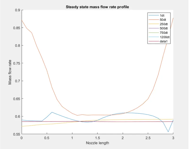
3. Mass flow rate distribution indiffrent time steps

Conservative

Non conservative

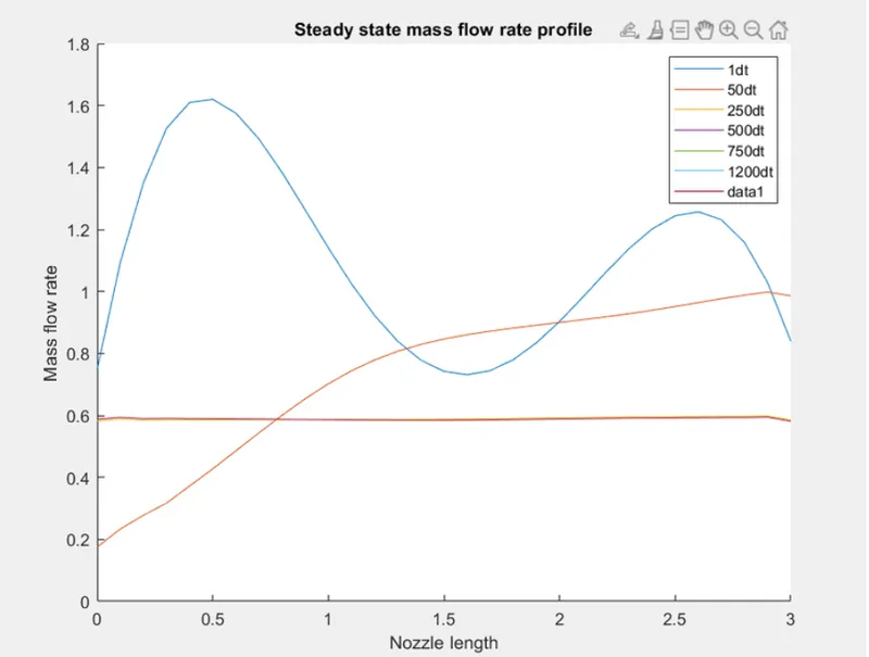
From the above plot, observed the mass flow rate of both forms, conservative and non conservative has diffrent types of initial conditions, the curve is closer to the analytical value more mass involved in conservative form , less mass involved in non convervative form.

Conclusion

• The conservative form yieds better mass flow distribution and it preserving the mass through the flow field. and the dependant variables in the non conservative form of the equations are primitive variables and the mass flow rate obtained.
• All the final solution of both form is similar. the non conservative form oscillation is more when it compared to conservative form
• Non conservative form leads to smaller residual amount which is used as index of quality to numerical algorithm
• Non conservative form gives slightly more accurate results for flow rate variables and the conservative form give more accurate values for flux variables
• Both Conservative and Non conservative forms are grid independant
• The Maccormack method provides stable and exact solution and we can solve various flows in this method.