Week 9 - FVM Literature Review
** Finite Volume Method:
1. Finite volume method is one of the methods in numerical computation in which the computational domain is divided into a number of infinitisimal volume (cells). Each cell has 1 cell centroid and 6 control surfaces which are also known as faces.
2. The centroid of each cell is called as grid point.
3. The computational discretized mesh is formed by joining the array of grid points.
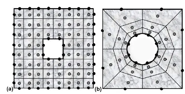
4. Each cell has a fixed volume. In case of 2D domain, the lateral side is assumed to be unity. In 2D mesh, each cell is assumed to have 4 control surfaces. Above figure represent the mesh generated in FVM method. Figure (a) represent uniform mesh in which the size of each cell is almost same. Figure (b) represent the non uniform mesh. Meshing can be done by considering 3 co-ordinate systems as per the geometry type. For orthogonal geometries, Cartesian type mesh is preferred while the geometries which have curvature, Cylindrical or spherical mesh is generated.
5. Conisder the following general scaler transport equation (Conservation of Energy)

The first term is volume integral of Temperature (Scalar) differential with respect to time. This integration is performed at the centroid of each cell. The second and third terms are area integrals. This integration is done at the face of each cell. The last term is also a volume integral which is calculated at cell centroid.
6. The finite-volume method’s strength is that it only needs to do flux evaluation for the cell boundaries. This also holds for nonlinear problems, which makes it extra powerful for robust handling of (nonlinear) conservation laws appearing in transport problems.
7. The local accuracy of the finite-volume method, such as close to a corner of interest, can be increased by refining the mesh around that corner
** Difference between FVM and FDM
| FVM | FDM |
| Suitable for complex geometries with irregular shape. | Not suitabel for complex geometries with irregular shape. |
| The computational domain is divided into number of cells which have infinitesimal volume. | The computational domain is divided into an array of nodes. There is no concept of cells. |
| Transport properties which are getting diffused or advected into the cells can be accurately analyzed. | The transport properties in integral form are converted into linear algebraic form and directly applied at node points. This compromises accuracy. |
| The physical laws are conservative in nature. FVM holds this property. | There isno such concept of censervation because FDM is just mathematical approach od solving differential equations. |
| Difficult to understand and implement. | Easy to understand and implement. |
| The curved boundaries do not create any problem since the cell shape at the boundary takes care of curvature effect in tranport property. | With the finite-difference method, we may easily run into problems handling curved boundaries for the purpose of defining the boundary conditions. |
| It can handle non linear problems. | Non linear problems are difficult |
| It can easily handle material discontinuities. | It is difficult to handle discontinuities in material using FDM. |
| Local grid refinement or adaptive grid refinement are possible. | Local or adaptive grid refinement is not possible. |
** Interpoltion Schemes **
* Need:
Consider the advection heat transfer problem in 2D
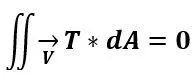
The above equation is discretized as
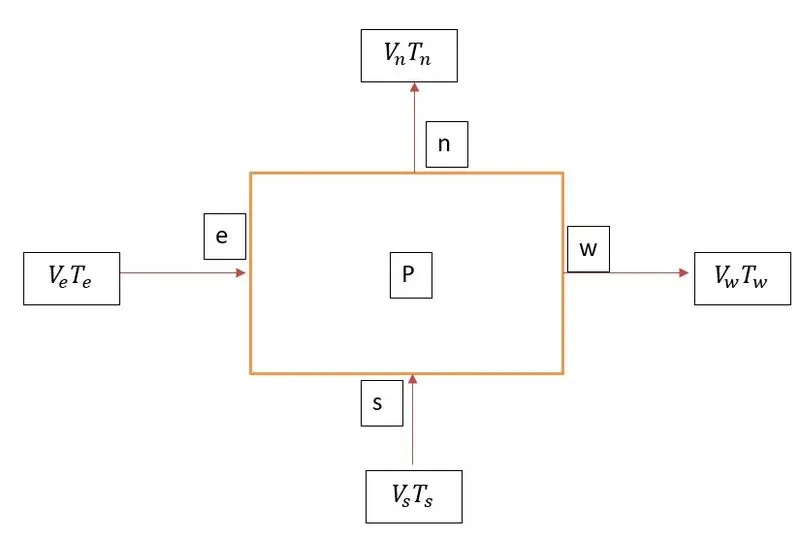
The intetgral form of equation is linearized as

The terms Te, Tw, Tn and Ts are obtained at face centers of east, west, north and south faces of cell with centroid P
To calculate these Temperature at faces, we need to use interpolation schemes
* There are 4 types of interpolation schemes
1. Central Difference Scheme
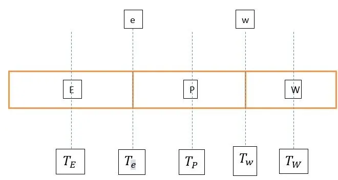
By this scheme, Te and Tw calculated as:
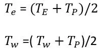
The central difference scheme has stability issues.
The scheme is unstable if value of cell Peclet Number : -2<= Pe<=2

2. First Order Upwind Scheme:
Upwind: Tail of arrow
Downwind: Head of wind
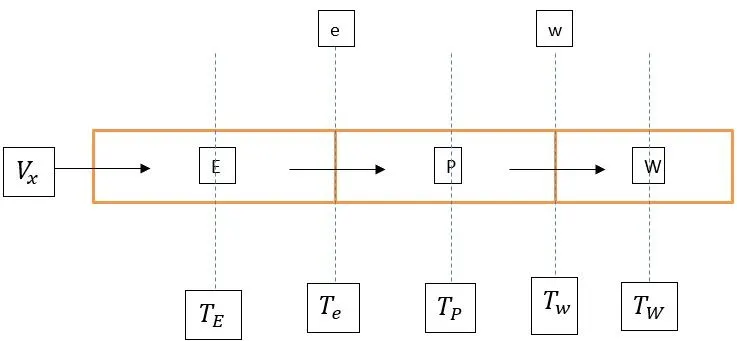
The values of Te and Tw are calculated as follows
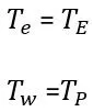
This scheme is inherently stable.
3. Second Order Upwind Scheme
In the case of uniform grid
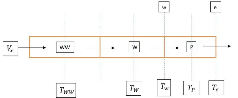
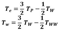
4. QUICK
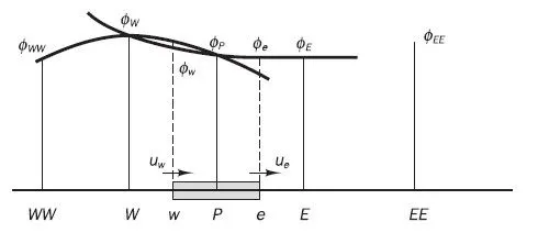
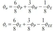
The quadratic upstream interpolation for convective kinetics (QUICK) scheme uses a three-point upstream-weighted quadratic interpolation for cell face values.
** Flux Limiters
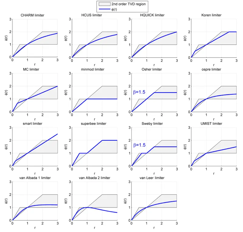
Flux limiters are used in high resolution schemes – numerical schemes used to solve problems in science and engineering, particularly fluid dynamics, described by partial differential equations (PDE's).
They are used in high resolution schemes, such as the MUSCL scheme, to avoid the spurious oscillations (wiggles) that would otherwise occur with high order spatial discretization schemes due to shocks, discontinuities or sharp changes in the solution domain.
The term flux limiter is used when the limiter acts on system fluxes.
Consider 1D semi discrete scheme

where
fluxes are represented as
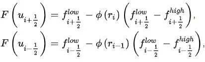
The following image shows how limiters reduce the wiggles and try to make solution as linear as possible.