Project 2 - Rankine cycle Simulator

Title: Simulation of Rankine Cycle

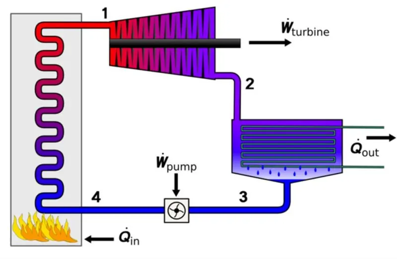
In rankine cycle the following processes occur

1-2: Isentropic compression in Turbine

2-3: Constant pressure heat rejection in Condenser

3-4: Isentropic compression using Pump

4-1: Constant pressure heat addition in Boiler

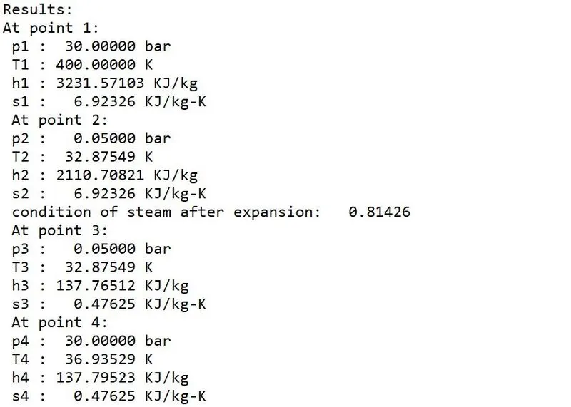
The conditions of steam at inlet of turbine (state point 1) is :

P1=30 bar and T1=400 deg.C

The condition of steam after expansion are:

P2=0.05 bar

We have "XSteam" library available with program. It contain thermodynamic properties of steam at different states.

So using this, we can find out values of various thermodynamic properties at different states.

The following is the way of extracting data from XSteam library.

enthalpy and entropy at state point 1 (at entry of turbine):
h1=XSteam('h_pT',p1,T1)
s1=XSteam('s_pT',p1,T1)

% for state point 2 (at exit of turbine):
% Let's assume point 2 lie within saturated vapor zone line inside the
% curve where dryness fraction is less than 1
s2=s1
% we have, s2=sf2+(x2*sfg2)
sf2=XSteam('sL_p',p2)
sg2=XSteam('sV_p',p2)
sfg2=sg2-sf2
x2=(s2-sf2)/(sg2-sf2)
% we know that, h2=hf2+(x2*hfg2)
hf2=XSteam('hL_p',p2)
hg2=XSteam('hV_p',p2)
hfg2=hg2-hf2
h2=hf2+(x2*hfg2)
if (x2<1)
    fprintf('Our assumption regarding location of state point 2 is correct')
else
    fprintf('State point 2 does not lie inside saturated vapour zone')
end

% enthalpy and entropy at state point 3 (at entry of pump):
h3=XSteam('hL_p',p2)     % since 2-3 is isobaric process, h3=hf2 (point 3 is on saturated liquid line)
s3=XSteam('sL_p',p2)     % since 2-3 is isobaric process, s3=sf2 (point 3 lies on saturated liquid line)
p3=p2
T3=XSteam('Tsat_p',p2)
T2=T3
v3=XSteam('vL_p',p2)

% enthalpy and entropy at state point 4:
s4=s3               % since 3-4 is isentropic process, s3=s4 
h4=h3+(v3*(p1-p2))    % use 1st law of thermodynamics
p4=p1

% Specific Steam consumption:
Sp_steam=3600/W_net

% Finding Cp and Cv
Cp=XSteam('Cp_ps',p4,s4)
Cv=XSteam('Cv_ps',p4,s4)
gama=Cp/Cv
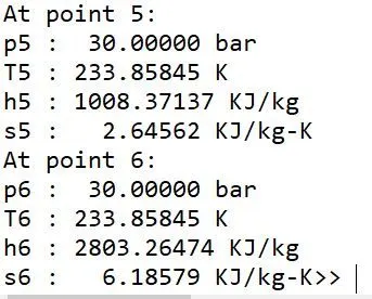
h5=XSteam('hL_p',p1)
u=p3/p4
q=(gama-1)/gama
T4=T3/(u^q)
p5=p4
h5=XSteam('hL_p',p1)
h6=XSteam('hV_p',p1)
s5=XSteam('sL_p',p1)
s6=XSteam('sV_p',p1)
T6=XSteam('Tsat_p',p1)
T5=T6
p6=p1

After obtaining values of different thermodynamic proerties at all desired points, we can find net work done and hermal efficieny of cycle as:

% Turbine work:
W_turb=h1-h2  % in KJ/kg

% Pump work:
W_pump= h4-h3 % in KJ/Kg

% Net work:
W_net= W_turb-W_pump   %in KJ/kg

% Heat supplied:
Qs=(h1-h4)*1000        %in KJ/kg

% Thermal efficiency:
efficiency=(W_net/Qs)*100

% Specific Steam consumption:
Sp_steam=3600/W_net    % kg/KW

% Plotting:

The plotting is done as follows:

1. T-S Diagram:

T=linspace(1,500,500)
for i=1:length(T)
    sf(i)=XSteam('sL_T',T(i))
    sg(i)=XSteam('sV_T',T(i))
    hf(i)=XSteam('hL_T',T(i))
    hg(i)=XSteam('hV_T',T(i))
end
% T-S Diagram:
figure(1)
hold on
plot(sf,T,'color','b','linewidth',2)
plot(sg,T,'color','b','linewidth',2)
plot([s1 s2],[T1 T2],'color','k','linewidth',2.5)
plot([s2 s3],[T2 T3],'color','k','linewidth',2.5)
plot([s3 s4],[T3 T4],'color','k','linewidth',2.5)
plot([s4 s5],[T4 T5],'color','k','linewidth',2.5)
plot([s5 s6],[T5 T6],'color','k','linewidth',2.5)
plot([s6 s1],[T6 T1],'color','k','linewidth',2.5)

sc1=linspace(s6,s1,500)
for j=1:length(sc1)
    Tc1(j)=XSteam('T_ps',p1,sc1(i));
end

title('Temperature vs Entropy')
xlabel('Entropy in KJ/Kg-K')
ylabel('Temperature in K')
legend('Saturation Curve')
text(s1+0.1,T1,'1')
text(s2+0.1,T2,'2')
text(s3-0.1,T3-30,'3')
text(s4,T4+20,'4')
text(s5-0.1,T5+20,'5')
text(s6,T6+30,'6')

2. H-S Diagram:

% H-S Diagram:
figure(2)
hold on
plot(sf,hf,'color','b','linewidth',2)
plot(sg,hg,'color','b','linewidth',2)
plot([s1 s2],[h1 h2],'color','k','linewidth',2.5)
plot([s2 s3],[h2 h3],'color','k','linewidth',2.5)
plot([s3 s4],[h3 h4],'color','k','linewidth',2.5)


hc=linspace(h3,h1,500)
for k=1:length(hc)
    S_c(k)=XSteam('s_ph',p1,hc(k))
end
plot(S_c,hc,'color','k','linewidth',2.5)
plot([s5 s6],[h5 h6],'color','k','linewidth',2.5)

for l=1:length(sc1)
    hc(l)=XSteam('h_ps',p1,entropy(l))
end


title('Entropy vs Enthalpy')
xlabel('Entropy')
ylabel('Enthalpy')
legend('Saturation Curve')
text(s1+0.1,h1,'1')
text(s2+0.1,h2,'2')
text(s3-0.1,h3-30,'3')
text(s4-0.1,h4+100,'4')
text(s5-0.1,h5+100,'5')
text(s6-0.1,h6+100,'6')

# Final Results: