Week 3.5 - Deriving 4th order approximation of a 2nd order derivative using Taylor Table method
** Taylor Table:
The general concept of Taylor table comes from the Numerical differentiation.
We know that,
f(x+h)=f(x)+h*f'(x)+h^2*f''(x)/2!+h^3*f'''(x)/3!+h^4*f''''(x)/4!+h^5*f'''''(x)/5!....
Now to find f'(x), we can modify above series
f'(x)=f(x+h)-f(x)/h - h*f''(x)/2! - h^2*f'''(x)/3!.....
In case of finding differentiation using Taylor's series we assume following general equation
Suppose we need to find 2nd order derivative of 'f' with respect to 'x' and we need 4th order accuracy
1. Central or Symmetric
First determine number of nodes to be selected on stencil.
We have P=N-Q+1
P is order of accuracy (P=4)
N is number of nodes
Q is order of derivative
So N=5
d^f/dx^2= a*f(i-2)+b*f(i-1)+c*f(i)+d*f(i+1)+e*f(i+2)
Now, expand each term using Taylor's series
f(i-2)= f(i)-2*f'(i)+2*f''(i)-(8*f'''(i)/6)+(16*f''''(i)/24)-(32*f'''''(i)/120)+(64*f''''''(i)/720)......
f(i-1)=f(i)-f'(i)+f''(i)/2-(f'''(i)/6)+(f''''(i)/24)-(f'''''(i)/120)+(f''''''(i)/720).......
f(i+1)=f(i)+f'(i)+f''(i)/2+(f'''(i)/6)+(f''''(i)/24)+(f'''''(i)/120)+(f''''''(i)/720).......
f(i+2)=f(i)+2*f'(i)+2*f''(i)+(8*f'''(i)/6)+(16*f''''(i)/24)+(32*f'''''(i)/120)+(64*f''''''(i)/720)......
Let's write all values in a tabulated form
| f(i) | dx*f'(i) | dx2*f''(x) | dx3*f'''(x) | dx4*f''''(x) | dx5*f'''''(x) | dx6*f''''''(x) | |
| a*f(i-2) | a | (-2)*a | 2a | (-8/6)*a | (16/24)*a | (-32/120)*a | (64/720)*a |
| b*f(i-1) | b | (-b) | b/2 | (-b)/6 | (b/24) | (-b/120) | (b/720) |
| c*f(i) | c | 0 | 0 | 0 | 0 | 0 | 0 |
| d*f(i+1) | d | d | d/2 | d/6 | d/24 | d/120 | d/720 |
| e*f(i+2) | e | 2*e | 2*e | (8/6)*e | (16/24)*e | (32/120)*e | (64/720)*e |
So now we obtain values of a,b,c,d,e by solving following equations
a+b+c+d+e=0
-2a-b+d+2e=0
4a+b+d+4e=2
-8a-6+d+8e=0
16a+b+d+16e=0
And we put the obtained values to get f''(x)
f''(x)=a*f(i-2)+b*f(i-1)+c*f(i)+d*f(i+1)+e*f(i+2)/(dx^2)
2. Left Skewed Scheme
P=4; Q=2
N=6 (we need 6 points on stencil)
d^f/dx^2=a*f(i-5)+b*f(i-4)+c*f(i-3)+d*f(i-2)+e*f(i-1)+f*f(i)
f(i-5)=f(i)-5*f'(i)+25/2*f''(i)-125/6*f'''(i)+625/24*f''''(i)-3125/120*f''''i(i)+15625/720*f''''''(i)......
f(i-4)=f(i)-4*f'(i)+16/2*f''(i)-64/6*f'''(i)+256/24*f''''(i)-1024/120*f'''''(i)+4096/720*f''''''(i)......
f(i-3)=f(i)-3*f'(i)+9/2*f''(i)-27/6*f'''(i)+81/24*f''''(i)-243/120-f'''''(i)+729/720*f''''''(i).......
f(i-2)= f(i)-2*f'(i)+2*f''(i)-(8*f'''(i)/6)+(16*f''''(i)/24)-(32*f'''''(i)/120)+(64*f''''''(i)/720)......
f(i-1)=f(i)-f'(i)+f''(i)/2-(f'''(i)/6)+(f''''(i)/24)-(f'''''(i)/120)+(f''''''(i)/720).......
Writing above equations in tabulated form
| f(i) | dx*f'(i) | dx2*f''(x) | dx3*f'''(x) | dx4*f''''(x) | dx5*f'''''(x) | dx6*f''''''(x) | |
| a*f(i-5) | a | 0 | 0 | 0 | 0 | 0 | |
| b*f(i-4) | b | (-b) | b/2 | (-b)/6 | (b/24) | (-b/120) | (b/720) |
| c*f(i-3) | c | (-2)*c | 2*c | (-8/6)*c | (16/24)*c | (-32/120)*c | (64/720)*c |
| d*f(i-2) | d | (-3)*d | (9/2)*d/ | (-27/6)*d | (81/24)*d | (-243/120)*d | (729/720)*d |
| e*f(i-1) | e | (-4)*e | (16/2)*e | (-64/6)*e | (256/24)*e | (-1024/120)*e | (4096/720)*e |
| f*f(i) | f | (-5)*f | (25/20*f | (-125/6)*f | (625/24)*f | (-3125/120)*f | (15625/7200*f |
solving following equations to get values of a,b,c,d,e,f
a+b+c+d+e=0
-b-2c-3d-4e-5f=0
b+4c+9d+16e+25f=2
-b-8c-27d-64e-125f=0
b+16c+81d+256e+625f=0
-b-32c-243d-1024e-3125f=0
3. Right Skewed Scheme:
P=4; Q=2
N=6 (we need 6 points on stencil)
d^f/dx^2=a*f(i)+b*f(i+1)+c*f(i+2)+d*f(i+3)+e*f(i+4)+f*f(i+5)
f(i+5)=f(i)+5*f'(i)+25/2*f''(i)+125/6*f'''(i)+625/24*f''''(i)+3125/120*f''''i(i)+15625/720*f''''''(i)......
f(i+4)=f(i)+4*f'(i)+16/2*f''(i)+64/6*f'''(i)+256/24*f''''(i)+1024/120*f'''''(i)+4096/720*f''''''(i)......
f(i+3)=f(i)+3*f'(i)+9/2*f''(i)+27/6*f'''(i)+81/24*f''''(i)+243/120-f'''''(i)+729/720*f''''''(i).......
f(i+2)= f(i)+2*f'(i)+2*f''(i)+(8*f'''(i)/6)+(16*f''''(i)/24)+(32*f'''''(i)/120)+(64*f''''''(i)/720)......
f(i+1)=f(i)+f'(i)+f''(i)/2+(f'''(i)/6)+(f''''(i)/24)+(f'''''(i)/120)+(f''''''(i)/720).......
Writing above equations in tabulated form
| f(i) | dx*f'(i) | dx2*f''(x) | dx3*f'''(x) | dx4*f''''(x) | dx5*f'''''(x) | dx6*f''''''(x) | |
| a*f(i) | a | 0 | 0 | 0 | 0 | 0 | |
| b*f(i+1) | b | (b) | b/2 | (b)/6 | (b/24) | (b/120) | (b/720) |
| c*f(i+2) | c | (2)*c | 2*c | (8/6)*c | (16/24)*c | (32/120)*c | (64/720)*c |
| d*f(i+3) | d | (3)*d | (9/2)*d/ | (27/6)*d | (81/24)*d | (243/120)*d | (729/720)*d |
| e*f(i+4) | e | (4)*e | (16/2)*e | (64/6)*e | (256/24)*e | (1024/120)*e | (4096/720)*e |
| f*f(i+5) | f | (5)*f | (25/20*f | (125/6)*f | (625/24)*f | (3125/120)*f | (15625/7200*f |
solving following equations to get values of a,b,c,d,e,f
a+b+c+d+e=0
b+2c+3d+4e+5f=0
b+4c+9d+16e+25f=2
b+8c+27d+64e+125f=0
b+16c+81d+256e+625f=0
b+32c+243d+1024e+3125f=0
** The following is the MATLAB code for Taylor Table:
Function is: exp(x)*cos(x)
dx=pi/6
clc
clear all
close all

% Function is: exp(x)*cos(x)
x = (pi/6);
dx = linspace(pi/40,pi/500,20);
analytical_derivative = -2*exp(x)*sin(x);


% Symmetric scheme:
% Let's assume 5 nodes such as: i-2,i-1,i,i+1,i+2
% d^2(f)/(dx^2)=a1*f(i-2)+b1*f(i-1)+c1*f(i)+d1*f(i+1)+e1*f(i+2)
% Solving set of linear equations
A1 = [1,1,1,1,1;-2,-1,0,1,2;4,1,0,1,4;-8,-1,0,1,8;16,1,0,1,16];
B1 = inv(A1);
C1 = [0;0;2;0;0];
D1 = B1*C1;

% Left skewed:
%d^(f)/(dx^2)=a2*f(i-5)+b2*f(i-4)+c2*f(i-3)+d2*f(i-2)+e2*f(i-1)+f2*f(i)
% A2 = [1,1,1,1,1,1;0,-1,-2,-3,-4,-5;0,1,4,9,16,25;0,-1,-8,-27,-64,-125;0,1,16,81,256,625;0,-1,-32,-243,-1024,-3125];
A2 = [1 1 1 1 1 1; -5 -4 -3 -2 -1 0; 25 16 9 4 1 0; -125 -64 -27 -8 -1 0; 625 256 81 16 1 0; -3125 -1024 -243 -32 -1 0];
B2 = inv(A2);
C2 = [0;0;2;0;0;0];
D2 = B2*C2;


% Right skewed:
% d^(f)/(dx^2)=a3*f(i)+b3*f(i+1)+c3*f(i+2)+d3*f(i+3)+e3*f(i+4)+f3*f(i+5)
% A3 = [1,1,1,1,1,1;0,1,2,3,4,5;0,1,4,9,16,25;0,1,8,27,64,125;0,1,16,81,256,625;0,1,32,246,1024,3125];
A3 = [1 1 1 1 1 1; 0 1 2 3  4 5; 0 1 4 9 16 25; 0 1 8 27 64 125; 0 1 16 81 256 625; 0 1 32 243 1024 3125];
B3 = inv(A3);
C3 = [0;0;2;0;0;0];
D3 = B3*C3;


for i=1:length(dx)
    % Central
    f_x1 = exp(x-(2*dx(i)))*cos(x-2*(dx(i)));
    f_x2 = exp(x-(dx(i)))*cos(x-(dx(i)));
    f_x3 = exp(x)*cos(x);
    f_x4 = exp(x+dx(i))*cos(x+dx(i));
    f_x5 = exp(x+(2*dx(i)))*cos(x+(2*dx(i)));

    % Left-Skewed
    f_y1 = exp(x-(5*dx(i)))*cos(x-(5*dx(i)));
    f_y2 = exp(x-(4*dx(i)))*cos(x-(4*dx(i)));
    f_y3 = exp(x-(3*dx(i)))*cos(x-(3*dx(i)));
    f_y4 = exp(x-(2*dx(i)))*cos(x-(2*dx(i)));
    f_y5 = exp(x-(1*dx(i)))*cos(x-(1*dx(i)));
    f_y6 = exp(x)*cos(x);

    % Right-Skewed
    f_z1 = exp(x)*cos(x);
    f_z2 = exp(x+(1*dx(i)))*cos(x+(1*dx(i)));
    f_z3 = exp(x+(2*dx(i)))*cos(x+(2*dx(i)));
    f_z4 = exp(x+(3*dx(i)))*cos(x+(3*dx(i)));
    f_z5 = exp(x+(4*dx(i)))*cos(x+(4*dx(i)));
    f_z6 = exp(x+(5*dx(i)))*cos(x+(5*dx(i)));

    DR2C(i)=(D1(1)*f_x1 + D1(2)*f_x2 + D1(3)*f_x3 + D1(4)*f_x4 + D1(5)*f_x5)/(dx(i)^2);
    DR2L(i)=(D2(1)*f_y1 + D2(2)*f_y2 + D2(3)*f_y3 + D2(4)*f_y4 + D2(5)*f_y5 + D2(6)*f_y6)/(dx(i)^2);
    DR2R(i)=(D3(1)*f_z1 + D3(2)*f_z2 + D3(3)*f_z3 + D3(4)*f_z4 + D3(5)*f_z5 + D3(6)*f_z6)/(dx(i)^2);

    error_symmetric(i) = abs(DR2C(i)-analytical_derivative);
    error_skew_left(i) = abs(DR2L(i)-analytical_derivative);
    error_skew_right(i)= abs(DR2R(i)-analytical_derivative);
end

figure(1)
loglog(dx,error_symmetric,'color','r','linewidth',1.5)
hold on
loglog(dx,error_skew_left,'color','b','linewidth',1)
hold on
loglog(dx,error_skew_right,'color','g')
xlabel('dx')
ylabel('error\_magnitude')
legend('symmetric','left\_skewed','right\_skewed')
After comparing the error, the following is the graph:
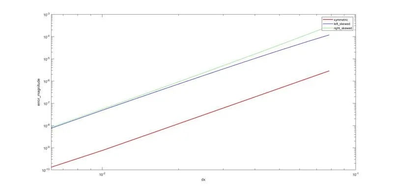
Comments: From the graph, it is seen that the best results are obtained by using symmetric scheme. For any values of dx say dx=0.02, the order of error magnitude in symmetric scheme is around 10^(-9) while in case of the right skewed scheme, is is in between 10^(-8) to 10^(-9) and same for left skewed scheme. So symmetric scheme is better.