Week 4.1 - Genetic Algorithm

• Optimization Process:

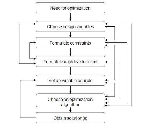
The first step is to identify need for optimization. In mechanical engineering, optimization means reducing the overall production cost as well as increasing the efficiecny or performance parameters of process.

Design variables are those design parameters which greatly affect the final result which can be in terms of performcance or cost. Example, material property could be a important design variable. If high ultimate strength material is used in design of shaft then dimension of shaft can be reduced as well as weigth of shft can be less by the use of material like alnico or titanium alloys but at the same time, its cost can slightly more.

Formulating constraints means determining the acceptable range of output values.

Then next step is formulating a mathematical replation between all variables.

Then we have to specify variable bound. Variable bound means restricting values of variables within a specified limit.

Then we have to select optimization algorithm. Genetic algorith is one of the most popular and most effective algorithms ever developed for optimization.

Genetic Algorithm:

Genetic algorithm (GA) is a metaheuristic inspired by the process of natural selection that belongs to the larger class of evolution algorith (EA). Genetic algorithms are commonly used to generate high-quality solutions to optimization and search problems by relying on biologically inspired operators such as mutation, crossover and selection.

In a genetic algorithm, a population of candidate solutions (called individuals, creatures) to an optimization problem is evolved toward better solutions. Each candidate solution has a set of properties (its chromosomes) which can be mutated and altered; traditionally, solutions are represented in binary as strings of 0s and 1s, but other encodings are also possible.

The evolution usually starts from a population of randomly generated individuals, and is an iterative process, with the population in each iteration called a generation. In each generation, the fitness of every individual in the population is evaluated; the fitness is usually the value of the objective function in the optimization problem being solved. The more fit individuals are stocastically selected from the current population, and each individual's genome is modified to form a new generation. The new generation of candidate solutions is then used in the next iteration of the algorithm.

Once the genetic representation and the fitness function are defined, a GA proceeds to initialize a population of solutions and then to improve it through repetitive application of the mutation, crossover, inversion and selection operators.

Initialization

The population size depends on the nature of the problem, but typically contains several hundreds or thousands of possible solutions. Often, the initial population is generated randomly, allowing the entire range of possible solutions. Occasionally, the solutions may be "seeded" in areas where optimal solutions are likely to be found.

Selection

During each successive generation, a portion of the existing population is selected to breed a new generation. Individual solutions are selected through a fitness-based process, where fitter solutions (as measured by a fittness function) are typically more likely to be selected. Certain selection methods rate the fitness of each solution and preferentially select the best solutions.

Genetic operators

crossover and mutation are combinedly known as genetic operators.

For each new solution to be produced, a pair of "parent" solutions is selected for breeding from the pool selected previously. By producing a "child" solution using the above methods of crossover and mutation, a new solution is created which typically shares many of the characteristics of its "parents". New parents are selected for each new child, and the process continues until a new population of solutions of appropriate size is generated.

Termination

This generational process is repeated until a termination condition has been reached. Common terminating conditions are:

• A solution is found that satisfies minimum criteria
• Fixed number of generations reached
• Allocated budget (computation time/money) reached
• The highest ranking solution's fitness is reaching or has reached a plateau such that successive iterations no longer produce better results
• Manual inspection
• Combination of all of the above.

Syntax for ga in MATLAB:

The following is syntax for ga

1. x = ga(fun,nvars) finds a local unconstrained minimum, x, to the objective function, fun. nvars is the dimension (number of design variables) of fun.
2. x = ga(fun,nvars,A,B,Aeq,Beq) finds a local minimum x to fun, subject to the linear equalities Aeq*x = beq and A*x ≤ b. (Set A=[] and b=[] if no linear inequalities exist.) ga evaluates the matrix product Aeq*x as if x is transposed (Aeq*x').
3. x = ga(fun,nvars,A,B,[],[],lb,ub) defines a set of lower and upper bounds on the design variables, x, so that a solution is found in the range lb ≤ x ≤ ub. (Set Aeq=[] and beq=[] if no linear equalities exist.)
4. x = ga(fun,nvars,A,B,[],[],lb,ub,nonlcon) subjects the minimization to the constraints defined in nonlcon. The function nonlcon accepts x and returns vectors C and Ceq, representing the nonlinear inequalities and equalities respectively. ga minimizes the fun such that C(x) ≤ 0 and Ceq(x) = 0. (Set lb=[] and ub=[] if no bounds exist.)
5. x = ga(fun,nvars,A,B,[],[],lb,ub,nonlcon,options) minimizes with the default optimization parameters replaced by values in options. (Set nonlcon=[] if no nonlinear constraints exist.) Create options using optimoptions.
6. x = ga(fun,nvars,A,B,[],[],lb,ub,nonlcon,Intcon) or x = ga(fun,nvars,A,b,[],[],lb,ub,nonlcon,IntCon,options) requires that the variables listed in IntCon take integer values.
7. x = ga(problem) finds the minimum for problem, a structure described in problem.
8. [x,fval] = ga(___), for any previous input arguments, also returns fval, the value of the fitness function at x.
9. [x,fval,exitflag,output] = ga(___) also returns exitflag, an integer identifying the reason the algorithm terminated, and output, a structure that contains output from each generation and other information about the performance of the algorithm.
10. [x,fval,exitflag,output,population,scores] = ga(___) also returns a matrix population, whose rows are the final population, and a vector scores, the scores of the final population

Explaination of code:

The function is:

function [f]=stalagmite_function(input_vector) 
f1x=(sin(5.1*pi*input_vector(1)+0.5))^6
f1y=(sin(5.1*pi*input_vector(2)+0.5))^6
f2x=exp((((input_vector(1)-0.0667)^2)/0.64).*(-4*log(2)))
f2y=exp((((input_vector(2)-0.0667)^2)/0.64).*(-4*log(2)))
f1=f1x*f1y*f2x*f2y;
f=-f1        % To maximize the objective function, multiply it with negative sign

The objective is to find the "maxima". Hence at the last, I have multiplied f1 with -ve sign to convert minima into maxima.

case1: Unbounded inputs:

clc
clear all
close all

tic
% Defining the research space:
x=linspace(0,0.6,150);            % x lies between 0 to 0.6
y=linspace(0,0.6,150);            % x lies between 0 to 0.6
num_cases=50;                     % we are running ga algorith for 50 times


% Creating 2D mesh:
[XX, YY]=meshgrid(x,y);

% case 1: Evaluating stalagmite function for unbounded search space:
for i=1:length(XX)                    % i 1 to 150
    for j=1:length(YY)                % j 1 to 150
        input_vector(1)=XX(i,j);      % input_vector(1) is matrix of values from x and y combine
        input_vector(2)=YY(i,j);      % input_vector(2) is matrix of values from x and y combine
        f(i,j)=stalagmite_function(input_vector);      % calling the stalagmite function
    end
end

tic
for k=1:num_cases
    [input,f_opt(k)]=ga(@stalagmite_function,2);       % HERE the function require 2 inputs
    x_opt(k)=input(1);
    y_opt(k)=input(2);
end
case1_time=toc;

figure(1)
subplot(2,1,1);                 % in subplot we have no. of iteratios vs max. value
surfc(XX,YY,-f);                % this si the main surface plot which has x,y and fval
xlabel('x values');
ylabel('y values');
title(' Finding maxima using stalagmite function for unbounded case');
shading interp
hold on
plot3(x_opt,y_opt,-f_opt,'marker','o','markersize',5,'markerfacecolor','r');
subplot(2,1,2);
plot(-f_opt);
xlabel('Number of iterations')
ylabel('Maximum value')
[inputs1,fval1]=ga(@stalagmite_function,2);

The output is:

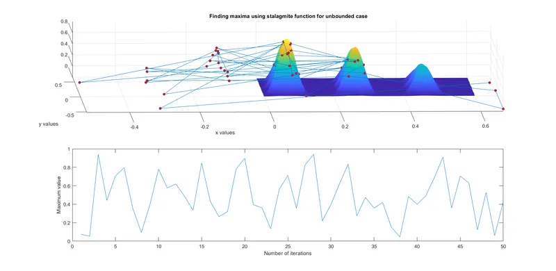
Explaination: Here we have specified range for x and y to be 0 to 0.6. But ga doesn't know this. Hence we can see some values less than 0 and some are grater than 0.6. This is wrong solution to optimization problem.

Case 2: Bounded inputs

% case 2: Evaluate stalagmite function with upper and lower bounds
tic
for k=1:num_cases
    [input,f_opt(k)]=ga(@stalagmite_function,2,[],[],[],[],[0;0],[1;1]);      % the null brackets indicate constraints.         % x bounds between 0 to 1 y bounds between 0 to 1
    x_opt(k)=input(1);
    y_opt(k)=input(2);
end
case2_time=toc;

figure(2)
subplot(2,1,1)
surfc(XX,YY,-f);
xlabel('x values (between 0 to 1)');
ylabel('y values (between 0 to 1)');
title(' Finding maxima using stalagmite function for bounded case ');
shading interp
hold on
plot3(x_opt,y_opt,-f_opt,'marker','o','markersize',7,'markerfacecolor','g');
subplot(2,1,2);
plot(-f_opt);
xlabel('Number of iterations')
ylabel('Maximum value')
[inputs2,fval2]=ga(@stalagmite_function,2);

Output:

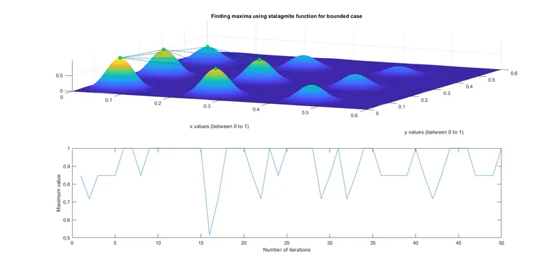
Explaination: Here we are restaining the limits of x and y to be 0 to 1. So ga takes vales for x and y between 0 to 1.

From the plot, we can see that maxima lies between x = 0 to 0.4 and y=0 to 0.5

Case 3:

% case 3: Increasing ga iterations:
options=optimoptions('ga');
options=optimoptions(options,'PopulationSize',170);

tic
for k=1:num_cases
    [input,f_opt(k)]=ga(@stalagmite_function,2,[],[],[],[],[0;0],[1;1],[],[],options);              % x bounds between 0 to 1 y bounds between 0 to 1
    x_opt(k)=input(1);
    y_opt(k)=input(2);
end
case3_time=toc;

figure(3)
subplot(2,1,1)
surfc(XX,YY,-f);
xlabel('x values (between 0 to 1)');
ylabel('y values (between 0 to 1)');
title(' Finding maxima using stalagmite function for bounded case with increases population ');
shading interp
hold on
plot3(x_opt,y_opt,-f_opt,'marker','o','markersize',7,'markerfacecolor','g');
subplot(2,1,2);
plot(-f_opt);
xlabel('Number of iterations')
ylabel('Maximum value')
[inputs3,fval3]=ga(@stalagmite_function,2);

Output:

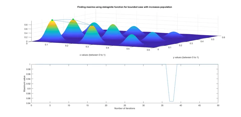
Explaination: Here we have increased the population size to 170. If population size is increased then the results tends to more accurate.

Case 4:

% case 4: Further increase in population size
    
options=optimoptions('ga');
options=optimoptions(options,'PopulationSize',300);

tic
for k=1:num_cases
    [input,f_opt(k)]=ga(@stalagmite_function,2,[],[],[],[],[0;0],[0.3;0.3],[],[],options);              % x bounds between 0 to 1 y bounds between 0 to 1
    x_opt(k)=input(1);
    y_opt(k)=input(2);
end
case4_time=toc;

figure(4)
subplot(2,1,1)
surfc(XX,YY,-f);
xlabel('x values (between 0 to 0.3)');
ylabel('y values (between 0 to 0.3)');
title(' Finding maxima using stalagmite function for bounded case with increases population ');
shading interp
hold on
plot3(x_opt,y_opt,-f_opt,'marker','o','markersize',7,'markerfacecolor','g');
subplot(2,1,2);
plot(-f_opt);
xlabel('Number of iterations')
ylabel('Maximum value')
[inputs4,fval4]=ga(@stalagmite_function,2);
total_time=toc;

output:

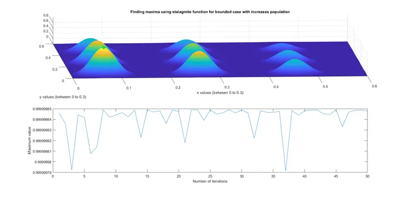
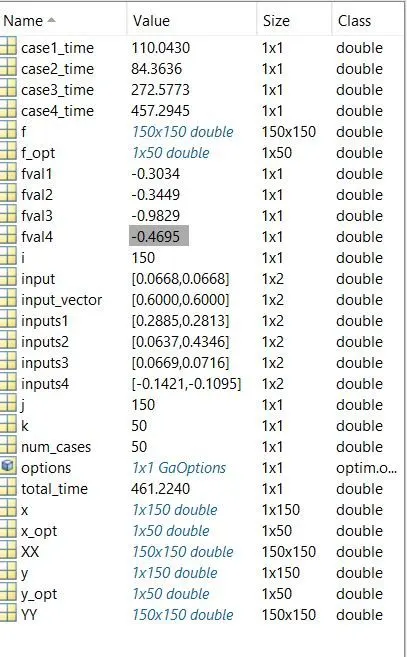
Explaination: The population size is increased from 170 to 300 and x and y limits are set to 0 to 0.3. So the global maxima is obtained.

Errors in code:

The above is the only error encountered during coding. This happened due to mentioning population option in case 2. It was corrected later.