Week 9 - FVM Literature Review

FINITE VOLUME METHOD:

The finite volume method (FVM) is a method for representing and evaluating partial differential equations in the form of algebraic equations. In the finite volume method, volume integrals in a partial differential equation that contain a divergence term are converted to surface integrals, using the divergence theorem. These terms are then evaluated as fluxes at the surfaces of each finite volume. Because the flux entering a given volume is identical to that leaving the adjacent volume, these methods are conservative. Another advantage of the finite volume method is that it is easily formulated to allow for unstructured meshes. The method is used in many computational fluid dynamics packages. "Finite volume" refers to the small volume surrounding each node point on a mesh.

In FVM instead of writing the equation in a single point, equations are written in an entire volume. It means for a considered volume no assumptions are made over the shape of the volume. Inside the particular volume, the flow is conserved, flow quantities are conserved, energy is conserved, mass is conserved, momentum is conserved, and so on. This is called 'Finite Volume Representation which begins with 'Integral form of governing equation':

Steps:

1. once we have this integral form of the equation.

2. Apply Gauss divergence theorem

3. We get discretized form which can be solved using a computer ("Flux Terms").

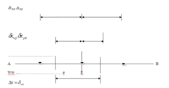
Step 1: Grid GenerationThe first step in the finite volume method is grid generation by dividing the domain into discrete control volumes. Let us place a number of nodal points in the space between A and B. The boundaries of control volumes are positioned mid-way between adjacent nodes. Thus each node is surrounded by a control volume or cell. It is common practice to set up control volumes near the edge of the domain in such a way that the physical boundaries coincide with the control volume boundaries. A general nodal point is defined by its neighbors in a one-dimensional geometry, the nodes to the west and east, are defined by W and E, respectively. The west face of the control volume is referred to by ‘w’ and the east side by ’e’. The distances of these points are given in figure

Step 2: DiscretizationThe most important feature of the finite volume method is the integration of the governing equation over a control volume to yield a discretized equation at its nodal points P.

Step 3: SolutionAfter discretization over each volume method, we are finding a system of an algebraic equation. Which are easily solved by numerical schemes such as Gauss-Siedel

2. MAJOR DIFFERENCE BETWEEN FINITE VOLUME METHOD AND FINITE DIFFERENCE METHOD:

• we cannot use FDM directly to a body whose grid points are not aligned properly along the x and y-direction. these may occur due to complex folds, cuts in the structure.
• as it is not aligned we cannot calculate the properties at the next adjacent point exactly, but we can make some correction factors and approximate it, this method is called the "Variable Transformation Method", which basically seeks to create a grid using different variable space which looks very similar to a cartesian grid.
• variable transformation method gives an approx solution of the property but it is time-consuming and complex
• for complex method this profile is less preferred

3. INTERPOLATION SCHEMES:

• The approximation of surface and volume integrals require the values of variables at locations other than the computational nodes of the control volume
• Values at these locations are obtained using interpolation
• Various interpolation schemes are

3.1. Upwind Interpolation (UDS)

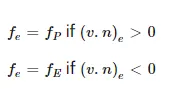
• UDS is equivalent to backward or forward difference approximation, depending on the flow direction
• The value of variable 'f' at the East face (e) is given by:

• It satisfies boundedness criteria unconditionally
• However, UDS is numerically diffusive

1. Diffusion is magnified if the flow is oblique to the grid in multi-dimensional problems

2. Large variations or peaks will be smeared out

• It is only first-order accurate and hence very fine grids are required to obtain an accurate solution

3.2 LINEAR INTERPOLATION(CDS):

• Approximates the value of the variable at CV face center by linear interpolation of the values at two nearest nodes
• It is equivalent to the central differencing formula for the first-order derivatives, and hence this is termed the Central Differencing

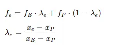
• CDS is second-order accurate on uniform grids, but formally of first order on a non-uniform grid
• Most widely used scheme as it results in simple approximations for the evaluation of gradients required for the evaluation of diffusive fluxes.
• however, it may produce an oscillating solution.

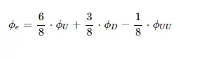
3.3 Quadratic Upwind Interpolation for Convective Kinematics (QUICK):

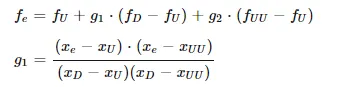
• Approximates the value of variable Tat CV face center by quadratic interpolation of the values at the three nearest computational nodes (one downstream (D) and two upstream (U, UU))
• It is third-order accurate for both uniform and non-uniform grids

3.4. Hybrid Interpolation Scheme:

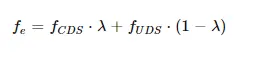
Blend of CDS and UDS scheme based on local Peclet number

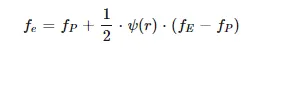
3.5 Total variation diminishing scheme(TVM):

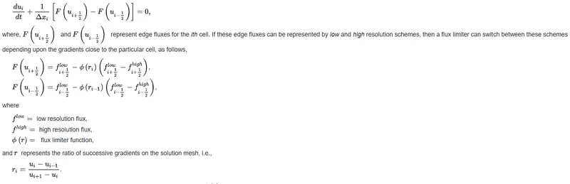
4. FLUX LIMITERS:

• Flux limiters are similar to slope limiters because they both have the same mathematical form, and both have the effect of limiting the solution gradient near shocks or discontinuities. In general, the term flux limiter is used when the limiter acts on system fluxes, and slope limiter is used when the limiter acts on system states (like pressure, velocity, etc.)
• It is commonly used in high-resolution schemes where the presence of discontinuities or shape variation is the solution domain may lead to oscillations that ruin the solution.
• It limits the spatial derivatives to realistic values and only operates when sharp wavefronts are present.
• these are commonly used in high-resolution schemes. It does not operate in smooth changing fluxes. these can be represented by higher-order approximations without introducing oscillations in the solution.

5. 1-D Linear steady-state heat conduction with a heat source

Assumptions

1. thermal conductivity is constants

2. Heat source is a linear function of temperature

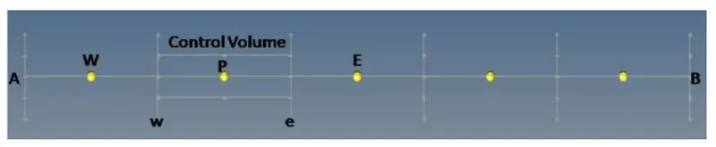
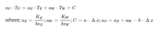
the domain is divided into several finite subdomains. Each subdomain is represented by a finite number of grid points. The governing differential equations should now be integrated over each subdomain. consider a profile assumption for the dependent variable for evaluating the above integrals to express them in terms of algebraic quantities at grid points.

discretization should satisfy:

1. physical consistency

2. overall balance

1-D steady-state heat equation:

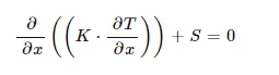
integrating over the control volume

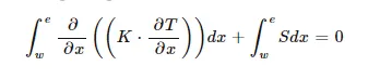
the source term is assumed to be a linear function of temperature

`s = (a+b.T)`

temperature distribution along the control volume can be assumed to be piecewise constant

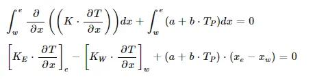
Gauss divergence theorem is used to convert volume integral to surface integral

temperature distribution for computation gradient cannot be assumed as piecewise constant, as this will result in zero temperature gradients. so we assume the temperature distribution to be price linear.

the above stone can be written as :