Week 5 - Rayleigh Taylor Instability

OBJECTIVE:

• some practical CFD models that have been based on the mathematical analysis of Rayleigh Taylor waves
• explain how these mathematical models have been adapted for CFD calculations.
• Perform the Rayleigh Taylor instability simulation for 2 different mesh sizes with the base mesh being 0.5 mm. Compare the results by showing the animations
• explain why a steady-state approach might not be suitable for these types of simulation.
• Run one more simulation with water and user-defined material(density = 400 kg/m³, viscosity = 0.001 kg/m-s) for refined mesh.
• Define the Atwood Number. Find out the Atwood number for both the cases and explain how the variation in Atwood number in the above two cases affects the behavior of the instability.

DESCRIPTION: The Rayleigh–Taylor instability or RT instability is the instability of an interface between two fluids of different densities which occurs when the lighter fluid is pushing the heavier fluid. Examples include the behavior of water suspended above oil in the gravity of Earth.

• CFD models that have been based on the mathematical analysis of Rayleigh Taylor waves are :

1. Kelvin Helmholtz instability: It is an instability that occurs when there is velocity shear in a single continuous fluid, or additionally where there is a velocity difference across the interface between two fluids. An example is a wind blowing over water: The instability manifests in waves on the water surface. More generally, clouds, the ocean, Saturn's bands, and the sun's corona show this instability.

2. Richtmyer - Meshkov instability: This instability occurs when two fluids of different densities are impulsively accelerated. normally this is by the passage of shock waves. The development of the instability beings with Small perturbations which initially grow linearly with time. This is followed by a non-linear regime with bubbles appearing in the case of light fluid penetrating a heavy fluid and with spikes appearing in the case of a heavy fluid penetrating light fluid. the difference across the interface between two fluids.

3. Plateau - Rayleigh instability: A liquid jet initially has a constant radius is falling vertically under gravity. The liquid length increases and reaches a critical value, At this critical value, the jet loses a stream of droplets. This phenomenon occurs primarily as a result of surface tension.

Practical CFD models:

SPH method(Smoother particle hydrodynaics)

Smoothed-particle hydrodynamics (SPH) is a computational method used for simulating the mechanics of continuum media, such as solid mechanics and fluid flows.Smoothed-particle hydrodynamics is being increasingly used to model fluid motion as well. This is due to several benefits over traditional grid-based techniques. First, SPH guarantees conservation of mass without extra computation since the particles themselves represent mass. Second, SPH computes pressure from weighted contributions of neighboring particles rather than by solving linear systems of equations. Finally, unlike grid-based techniques, which must track fluid boundaries, SPH creates a free surface for two-phase interacting fluids directly since the particles represent the denser fluid and empty space represents the lighter fluid.

SINGLE-FLUID MODEL

A typical approach used for the analysis of two-phase flows is a mixture model, i.e. the individual fluid phases are assumed to behave as a flowing mixture described in terms of the mixture properties. The applied single-fluid model is a five-equation model consisting of the mass, momentum and energy equations for a vapor/liquid mixture, and two equations describing the formation and growth of the liquid phase.

TWO-FLUID MODEL

In the two-fluid model, separate sets of the governing equation for the vapor and liquid phases have been used. The interaction between the droplets and the heat exchange between the liquid phase and the solid boundary are not modelled here as well. Additionally, the velocity slip between vapor and the liquid phase is in this model taken into account.

Turbulence model

Turbulence models are needed to predict the average mixing behaviour in flows that are on average one- or two-dimensional. The approach to the construction of tile turbulence model is guided by the experimental behaviour.The equations governing turbulent flows can only be solved directly for simple cases of flow. For most real life turbulent flows, CFD simulation use turbulent models to predict the evolution of turbulence. These turbulence models are simplified constitutive equations that predict the statistical evolution of turbulent flows.

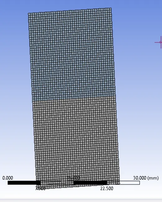
CASE:1 MESH ELEMENT SIZE:0.5mm

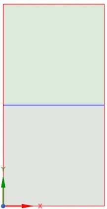
MESH:

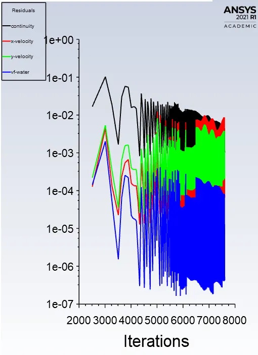
RESIDUAL:

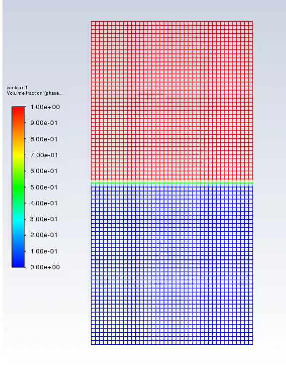
SIMULATION VIDEO:

https://youtu.be/D5Lid8Ba9b8https://youtu.be/EqnhCGgVeyQ

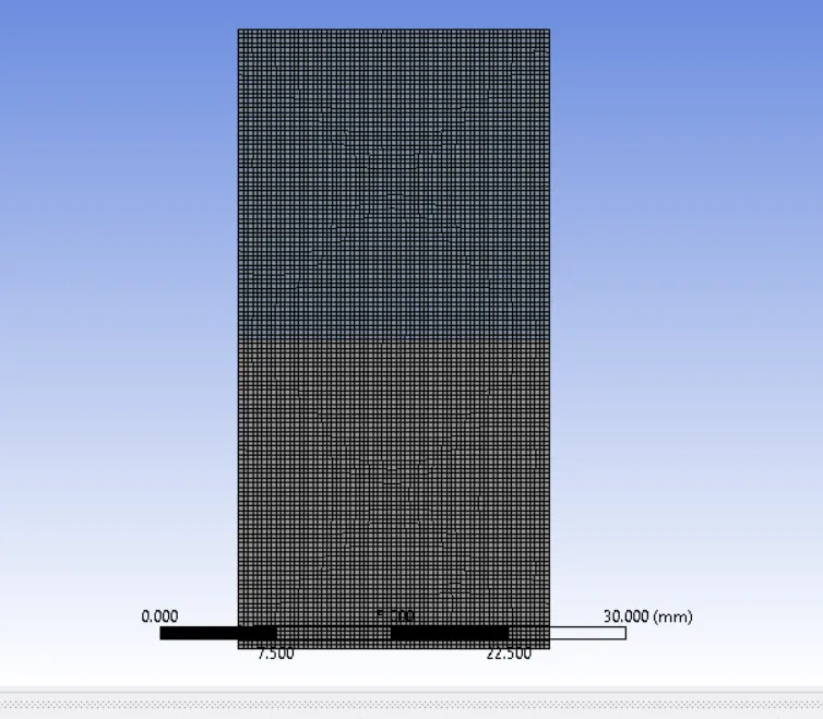
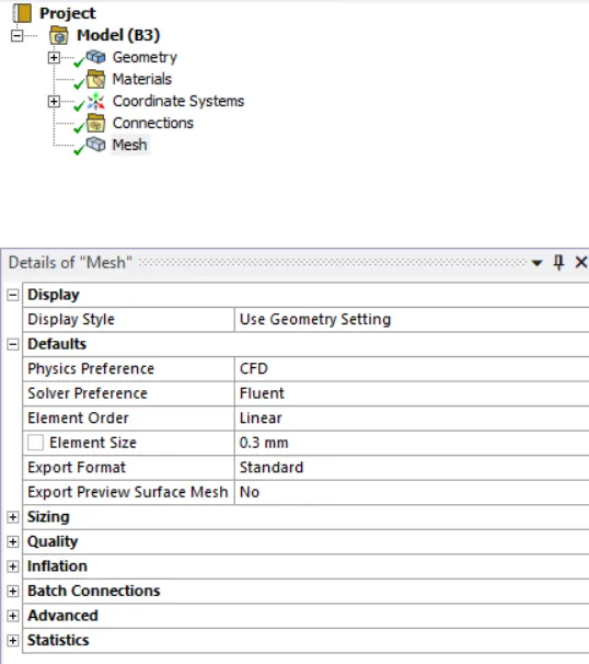
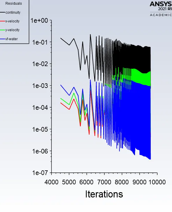
CASE:2 mesh elemetn size : 0.3mm

RESIDUAL:

SIMULATION VIDEO LINK:

https://youtu.be/29wKAAvIyq0

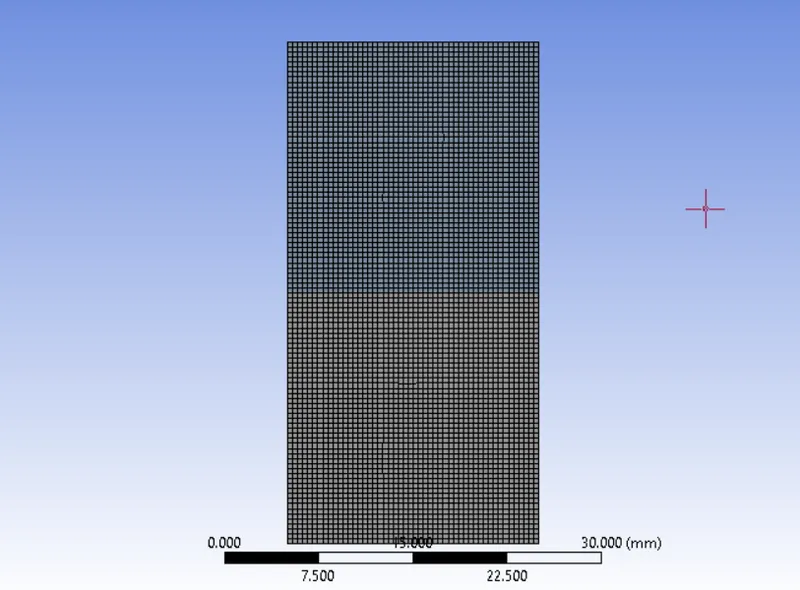
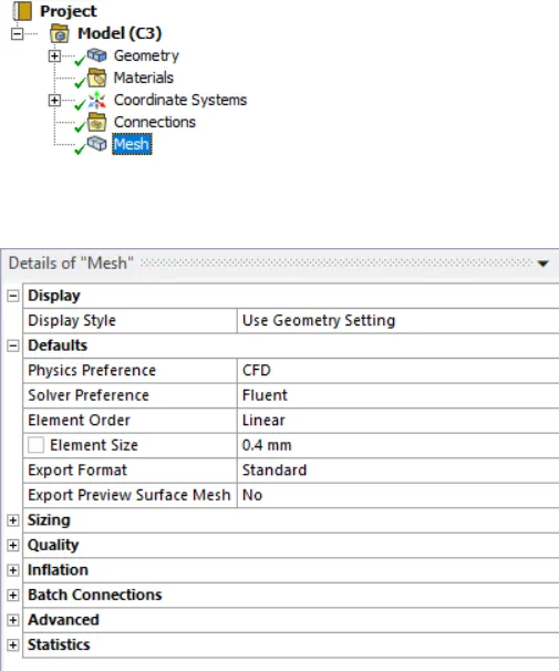
CASE:3 MESH ELEMENT SIZE : 0.4mm

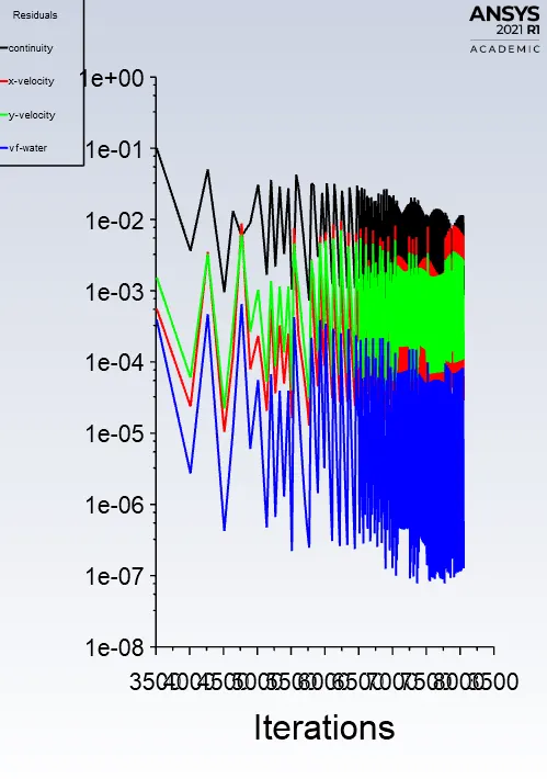
RESIDUAL:

SIMULATIONS VIDEO:

https://youtu.be/QzoGYgQpQz8

CASE:4 MESH ELEMENT SIZE: 0.3mm with water and userdefined material

MESH:

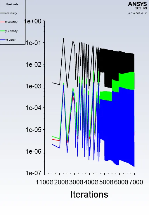
RESIDUALS:

SIMULTION VIDEO:

https://youtu.be/fvpY8EXhEt0https://youtu.be/y99j_TGRQik

OBSERVATION

In the above cases, the simulation starts with the state of hydrostatic equilibrium and the Rayleigh Taylor instability is observed at the interference when a lower density fluid pushes a higher density fluid due to which formation of shock waves at the interface takes place. Formation of air bubbles starts taking place, which compresses the heavy fluid around it, due to which shock waves of multidimensional fashion generates and it gets more stronger as it moves upward.

It is observed that the more we refine the mesh, the more the simulation results get smoother about the irregularities that take place at the interface of the two fluids. As higher density fluid replaces lower density fluid, the formation of air bubbles and vortex takes place, which travels towards the upward region with time. In case-3, we can see the more detail results about the formation of waves and the formation of some air bubbles that get trapped at the lower region during the initial stage and then they travel towards the upper region, generating shock waves. At the end of the simulation, it is to be observed that the two phases get separated from each other though, we can see some diffusivity between them which is a volume fraction of air and water.

why a steady-state approach might not be suitable for the above types of simulation?

The difference between the steady and transient is that you can't see the small-time variation of instability. The steady-state simulation is performed if we are concerned more about the final state results or the equilibrium state. In RT-Instability CFD models, we are more concerned to learn about the transition of the irregularities that starts developing when we pour high dense fluid upon low dense fluid under gravity effect so, by using transient solver along with refined mesh of the model, we can compute the smooth transition of irregularities that takes place at the interface of the fluids. The final state results for both the steady-state and transient state will be the same.

In this probleem we are observing the instabilities when it is occuring so we are not concerened about the final answer because steady state is more into caapturing the final results but by transient we can see the behaviour of the solution and every instant such that capturing bubbles,vortec and shockwaves. so this is reason why transient is more suitable than steady state model

• ATWOOD NUMBER: The Atwood number (A) is a dimensionless number in fluid dynamics used in the study of hydrodynamic instability in density stratified flows. It is a dimensionless density ratio defined as

where ρ1 is the density of the higher fluid

and ρ2 is the density of the lighter fluid

A = (1000 - 1.25) / (1000 + 1.25) = 0.9975

Atwood number is an important parameter in the study of Rayleigh-Taylor instability. For Atwood number close to 0, RT instability flows take the form of asymmetric “finger” of fluid; for Atwood number close to 1, the much lighter fluid “below” the heavier fluid takes the form of larger bubble-like plumes.

The calculated Atwood number is close to 1 and from the simulation results, it is found that when high dense fluid i.e. water poured upon low dense fluid i.e. air under gravity, the formation of air bubble-like plumes takes place which travels towards the upward region in the form of waves and some gets trapped at the lower regions during the initial stages, which afterward try to move towards the upper region and at the end, both phases gets separated with some diffusivity left at the middle portion between them. Thus, the calculated Atwood number is validated for our simulation results.

For above cases

case 1:

heavier fluid(water)

density 1=998.2 kg/m^3

lighter fluid(air)

density 2=1.225 kg/m^3

Atwood number(A) =(density 1-density2)/(density 1+density2)

Atwood number(A)=0.996

case 2:

heavier fluid(water)

density 1=998.2 kg/m^3

lighter fluid(user-defined material)

density 2=400 kg/m^3

Atwood number(A) =(density 1-density2)/(density 1+density2)

Atwood number(A)=0.427

variation in Atwood number in the above two cases affects the behavior of the instability.

For Atwood numbers close to 0, RT instability flows take the form of symmetric figures of fluid.

When Atwood number is close to 1, the much lighter fluid below the heavier fluid takes the form of larger bubble-like plumes.

Therefore, from the value of Atwood number, it is seen from the simulations that air forms larger bubbles when water is poured down the air pushes through and forms large bubbles. Therefore, the results can be validated by obtaining the value of the Atwood number.

Atwood number is an important parameter in the body of Rayleigh Taylor instability and Richtmyer-Meshkov instability. In Rayleigh-Taylor instability, the penetration distance of heavy fluid bubbles into the lighter fluid is a function of the acceleration time scale. A*g*t^2, where 'g' is the acceleration due to gravity and 't' is the time.

Atwood number effects on the instability of a uniform interface driven by a perturbed shock wave and Rayleigh Taylor instability:-

The evaluation of a uniform interface subjected to a perturbed shock wave has been experimentally studied over a range of Atwood numbers 0.22 <= A <= 0.68 and Mach numbers 1.2 <= M <= 1.8 using a vertical shock tube. The perturbed shock wave is produced by diffracting a planar incident shock over a rigid cylinder. The wave patterns of the perturbed shock are captured by high-speed shadowgraphy while the evolution of the shock interface is captured by planar Mie scattering. Besides the formation of a cavity and two steps, an apparent counter-rotating vortex pair emerges on the shock interface due to the baroclinic vorticity deposition, as both the Atwood number and Mach number increase, Quantitatively it is interesting to note that the amplitude growth rate of the shocked interface decreases with increasing the Atwood number, which is fundamentally different from the results related to the classical RM instability. This notable feature is explained by the approximation of an oblique shock hitting a uniform interface. For weak shock, a suitable time scaling is employed to collapse experimental data irrespective of the Atwood number difference.