Week 9 - FVM Literature Review

WEEK 9 - FVM LITERATURE REVIEW

OBJECTIVES:

• To explain the finite volume method.
• To compare between FDM and FVM.
• To describe the need for interpolation schemes in FVM.
• To describe the flux limiters in FVM.

FINITE VOLUME METHOD:

Introduction:

• The Finite Volume Method (FVM) is a method for representing and evaluating partial differential equations in the form of algebraic equations.
• Finite volume method (FVM), like FEM, is based on an unstructured (e.g. triangular) mesh. Therefore, it is suitable for irregular and complex geometries.
• FVM is based on the integral form of the conservation laws, rather than their differential form. This leads to more accuracy/stability, especially for sharp gradients (i.e. large derivatives) inside a domain, which is also called shock-capturing property.

Procedure:

• FVM can be used on all differential equations, which can be written in the divergence form. This effectively writes the equation using divergence operators.
• The equation is then integrated over the volume. We can then apply Gauss’s theorem converting the volume integral over the divergence into a surface integral across the boundaries.
• The integral is therefore turned from integrating the differential of the dependent variable inside of the cells into surface integrals of the fluxes of the dependent variable across the boundary of the cells.
• These integrals can usually be calculated using suitable numerical approximation methods. This simplifies the differential equation substantially.

Let us take an example, the differential form of the continuity equation can be written as

`(del rho)/(del t) + (del (rho u))/(del x) + (del (rho v))/(del y) + (del (rho w))/(del z)`

where u, v, and w are the components of flow velocities in the x, y, and z directions, and ρ is the density.

The integral form of continuity for a control volume can be written as

`del/(delt) int_v rho**dV + intrhou*dS = 0`

where V is the control volume, S is the control surface, u = (u, v, w), and S is the surface vector.

Therefore, the change of mass inside a control/finite volume plus the net mass fluxes through the control surface should be zero. In FVM, the domain is first discretized into a number of nonoverlapping finite volumes or cells. Usually, these finite volumes are triangles (2D) or prisms (3D). Next, conservation laws are applied to each individual cell to form enough algebraic equations, which can be solved to compute the state variables.

ADVANTAGES OF FVM:

1. un-structured grids:

• There are no requirements on the grid to be structured (although structured grids can still be used). The Finite Volume Method is therefore suitable for complex geometries.
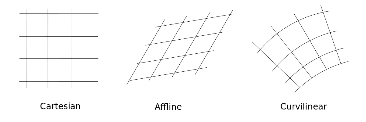
• For 2D, Structured Grid means Quadrilateral i.e.

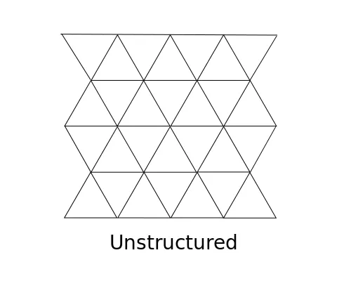
• For 2D, Unstructured Grid means Triangle i.e.

2. Computational efficiency:

• Structured grids are less computationally efficient than unstructured grids, because of the rigid connectivity restriction.
• This resitrction may require high grid density where low grid density is needed - but this is dependent on the particular case.

3. Memory requirements

• However, for the same number of grid points, structured grids require less memory to store than unstructured grids, because of the simpler connectivity.

4. Convergence

• Structured grids may allow better convergence and higher resolution than unstructured grids and therefore higher accuracy, as the rigid connectivity limits the possibility for skewed elements.

5. Geometry complexity

• Unstructured grids are more suited for highly complex geometries, whereas structured grids are better suited to simple geometries.

COMPARISION BETWEEN FDM AND FVM:

• FDM is a differential scheme, that is approximation of a taylor series expansion. We write the first order, second order differential in terms of difference between two point values. This may bring in some approximation error.
• Finite Volume method is an integral scheme. Since you are integrating across the area, chance of error is minimized.
• By, comparing differential and an integral scheme integral scheme is better in terms of error.
• Differential schemes are faster and error can be minimized if you have regular grids (squares and rectangles).
• Integral schemes are slightly slower but score over FDM when the mesh is irregular.

NEED FOR INTERPOLATION SCHEMES:

• The interpolation schemes in FVM are required for the conversion of integral form of the governing equation to an algebraic equation which can then be solved using various numerical methods.
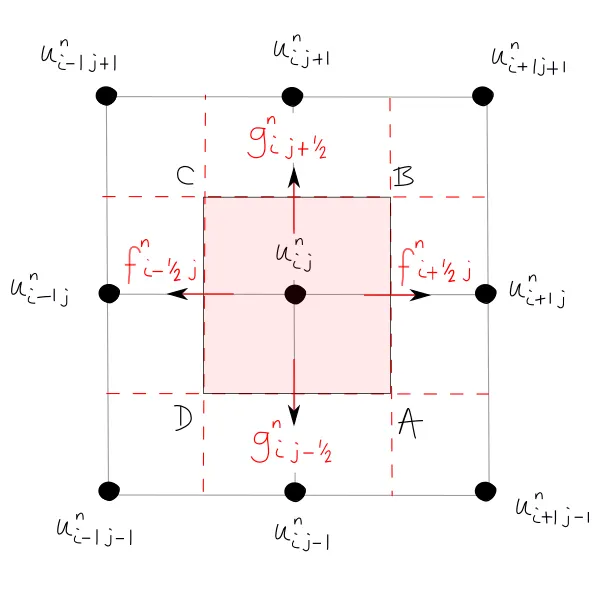
• The use of interpolation schemes to approximate the property values located at the boundaries of the control volumes are necessary when FVM is applied, using as interpolation nodes the correspondent properties located at the center of the adjacent control volumes.

Types of interpolation schemes:

• Linear interpolation
• Upwind interpolation
• Quadratic Upwind Interpolation Scheme (QUICK)
• Hybrid

1. TVD (Total Variation Dimension)

2. ENO (Essentially Non Oscillatory)

FLUX LIMITERS IN FVM:

Flux limiters are used in high resolution schemes – numerical schemes used to solve problems in science and engineering, particularly fluid dynamics, described by partial differential equations (PDE's). They are used in high resolution schemes, such as the MUSCL scheme, to avoid the spurious oscillations (wiggles) that would otherwise occur with high order spatial discretization schemes due to shocks, discontinuities or sharp changes in the solution domain. Use of flux limiters, together with an appropriate high resolution scheme, make the solutions total variation diminishing (TVD).

Note that flux limiters are also referred to as slope limiters because they both have the same mathematical form, and both have the effect of limiting the solution gradient near shocks or discontinuities. In general, the term flux limiter is used when the limiter acts on system fluxes, and slope limiter is used when the limiter acts on system states (like pressure, velocity etc.).

Working principle:

• The main idea behind the construction of flux limiter schemes is to limit the spatial derivatives to realistic values – for scientific and engineering problems this usually means physically realisable and meaningful values.
• They are used in high resolution schemes for solving problems described by PDEs and only come into operation when sharp wave fronts are present.
• For smoothly changing waves, the flux limiters do not operate and the spatial derivatives can be represented by higher order approximations without introducing spurious oscillations.